The goal of this week's lab is to have you implement two popular algorithms for tree inference: Neighbor Joining (an example of distance-based methods) and Weighted Parsimony (an example of character-based parsimony methods) and visualize the results. You may work with a lab partner on this lab and use either Python or C++ for your implementation

We will be doing the following problems in-lab. Given the matrix in your labs/NJTree directory titled inclass.dist:

1. Demonstrate whether the matrix is ultrametric or not
2. Demonstrate whether the matrix is additive
3. Run the UPGMA algorithm on the distance matrix
4. Run the neighbor joining algorithm

Neighbor Joining is the most popular distance-based method for inferring tree structures given its ability to handle non-ultrametric data. You will write a program NJTree that will output a list of edges formed in the tree. Your program should take in one command line argument for a file containing your distance values. An example run for a Python program would be:

$ ./NJTree.py distances

Your distance file will be in the format:

A B distance_AB

with one line for each pair of taxa in the set. Since distances are symmetric, the ordering of the sequences is not important.

To name your clusters, simply merge the names of the two sub-clusters with a hyphen in between, e.g. merging A and B yields A-B

Note: The expected output has changed since the original posting: Your program should output a list of edges in your tree in a similar format.

A A-B distance_AA-B
B A-B distance_BA-B

In addition, should output a visualization of your tree using the instructions below.

Visualize Tree using GraphViz

You should construct a visualization of your unrooted tree using GraphViz. To do so, firs import the Python GraphViz library

import pygraphviz as pgv

To create a graph G and add nodes and edges:

G = pgv.AGraph() #Constructs a graph object
G.add_node("A")
G.add_node("B")
G.add_edge("A","B",label="1.0", len=1.0)

You will add a node for each sequence in the set. Then, every time a cluster is created by merging two smaller clusters, you will create a node for that cluster and add edges to the two merged clusters. For each edge, both the label and len should be the distance, d_ik between the two clusters i and k. I suggest setting the len field to a minimum value of 1.0 to overcome overlapping nodes. When you finish the main loop, you will merge your last two clusters by adding an edge. Lastly, you will output your graph to a file by using the command:

G.draw("tree.png",prog="neato")  

You can use your favorite image viewer to view your results.

Sample Output

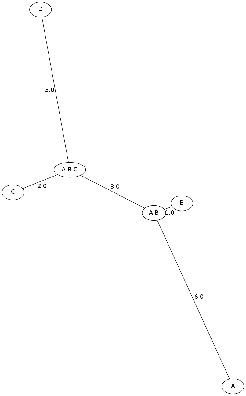
Using the in-lab example (run update68 to obtain inclass.dist)

$ ./NJTree.py inclass.dist
A A-B 6.0
B A-B 1.0
A-B A-B-C 3.0
C A-B-C 2.0
D A-B-C 5.0

The resulting image: In-class Example

Analysis

You should see an input file primate.dist in your directory. Run your program on this matrix and submit the resulting png as primate.png in the supl directory. These distances are scaled distances of mitochondrial DNA found in several organisms. I have abbreviated the names to avoid large node sizes in GraphViz. The mapping is as follows:

• G: Gorilla
• H: Human
• B: Gibbon
• C: Chimpanzee
• O: Orangutan

In my mailbox, hand in written (or typed) solutions to the following questions:

1. Which two species were joined first by the neighbor-joining algorithm?
2. Are these two species the closest pair of species in your data set according to the original distance matrix?
3. If so, explain why the algorithm guarantees this result. If not, explain why this pair was chosen first

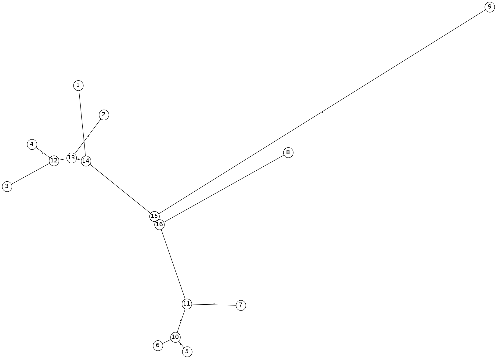
For the next set of questions, take a look at the following image produced by the neighbor joining algorithm for studying HIV. The numbers in the nodes map to various strains of HIV (human immunodeficiency virus) and SIV (simian immunodeficiency virus). You can take a look at the mapping and original distance matrix.

AIDS (Acquired Immune Deficiency Syndrome) is caused by two variants of HIV in humans - HIV-1 and HIV-2. You will use the tree to answer questions about the evolution of these two variants, in particular focusing on their relationship with various strains of SIV.



4. Taking a look at the graph and provided mapping, which virus strain is the outgroup?
5. Draw a rooted tree using your answer to the previous question. Do not worry about drawing branch lengths to scale, but the resulting topology must match the unrooted tree.
6. Given the tree you have produced, draw some rough conclusions about the evolution of HIV-1 and HIV-2. Does it appear that they evolved from one common simian source or independently from different simian groups? HINT: are the two strains more closely related to each other/a common ancestor than all other strains of SIV? If so, they probably recently developed from the same/similar ancestor. If not, they are more likely independent paths.

For the second part of your lab, you will implement the Weighted Parsimony method detailed in class. Your program will take in a tree, a scoring function, and the sequences of the leaf nodes and outputs a score for the tree and assigned labels inferred for the ancestral nodes.

$ ./weightedParsimony.py tree substitution_matrix leaf_sequences

Input Files

Leaf Sequences: Contains a list of all of the K sequences you are attempting to line up in the phylogenetic tree. Each line will be in the format:

identifier: sequence

The identifier should be the same name you use when defining the tree (below). Using the example we have from class, I have labeled each leaf sequence as L1 through L4 in weightedParsimony/inclass.seq

L1: A
L2: C
L3: T
L4: G

Tree File: The tree file will define the topology of the phylogenetic tree you are attempting to score. The first line specifies the root. Each line after that is in the format:

child parent

For example, the simple tree from class (weightedParsimony/inclass.tree) would be:

N1
N2 N1
N3 N1
L1 N2
L2 N2
L3 N3
L4 N3

Note that the root has been labeled N1. It has two children N2,N3. The leaves connect to either N2 or N3.

Weight Matrix: Specifies the substitution value for each pair of states possible at each position in the sequence. This has the exact same format as the distance matrix in the Neighbor Joining algorithm; that is, each line contains a pair of characters followed by their substitution score. You can find the example from class in weightedParsimony/inclass.wgt:

A C 9
A G 4
A T 3
C G 4
C T 4
G T 2

The diagnol is not defined, but you should set it to 0 when you create your substitution function.

Output

Your program should print the total tree score as well as the inferred state of all common ancestors after running the weighted parimony algorithm. Each line should be specified as:

identifier: sequence

similar to the input sequence file. The in-lecture example would appear as follows (I have shown intermediate values for debugging purposes, you are only required to output the data below the asteriks):

$./weightedParsimony.py inclass.tree inclass.wgt inclass.seq 
L4 : A : (100000.0, None, None)
C : (100000.0, None, None)
T : (100000.0, None, None)
G : (0.0, None, None)

L2 : A : (100000.0, None, None)
C : (0.0, None, None)
T : (100000.0, None, None)
G : (100000.0, None, None)

L3 : A : (100000.0, None, None)
C : (100000.0, None, None)
T : (0.0, None, None)
G : (100000.0, None, None)

L1 : A : (0.0, None, None)
C : (100000.0, None, None)
T : (100000.0, None, None)
G : (100000.0, None, None)

N1 : A : (14.0, A, T)
C : (15.0, C, T)
T : (9.0, T, T)
G : (10.0, G, G)

N2 : A : (9.0, A, C)
C : (9.0, A, C)
T : (7.0, A, C)
G : (8.0, A, C)

N3 : A : (7.0, T, G)
C : (8.0, T, G)
T : (2.0, T, G)
G : (2.0, T, G)

*********************************

Score: 9.0

Inferred States: 
L4: G
L2: C
L3: T
L1: A
N1: T
N2: T
N3: T

Trees

While you can construct a Tree data structure to help implement your program, it is probably much easier to just use a dictionary instead. For example you can have a dictionary where the key is the identifier (e.g., "N1") and the value is a list of the children (e.g., ["N2","N3"]). A leaf node simply has an empty list for its value.

Real sequences

You should first get your program to work on single-character sequences as practiced in class. Once that is complete, you will want to improve your algorithm to calculate the cumulative score and trace for a set of sequences of length N. You can assume that each leaf sequence is of the same length. Also, since we assume independence of positions, you should be able to just place a loop around your existing code repeating the calculation for each position in the sequence, u. I have given a second set of example files beginning with the prefix long. A sample run will output:

$./weightedParsimony.py long.tree long.wgt long.seq 
Score: 11.0

Inferred States: 
Aardvark: CAGGTA
Chimp: CGGGTA
Dog: TGCACT
Bison: CAGACA
Elephant: TGCGTA
C3: CGGGTA
C2: TGCGTA
C1: CAGGTA
C4: CGCGTA

An output of intermediate values can be found here.

When you are finished with your lab, submit your code using handin68. You should submit, at a minimum:

1. NJTree.py and associated source code in the NJTree directory.
2. primate.png showing your solution to neighbor joining on the primate mitochondrial DNA in the supl directory
3. The answer to the analysis questions in hard copy in the mailbox outside my office.
4. weightedParsimony.py and associated source code in the WeightedParsimony directory.

Home Page