Lab 03

Writeup

As you go along, be sure to be updating your Writeup.md file with answers to questions!

GloVe vectors

“GloVe is an unsupervised learning algorithm for obtaining vector representations for words.” (Jeffrey Pennington, Richard Socher, and Christopher D. Manning. 2014. Global Vectors for Word Representation)

The GloVe algorithm takes a large text corpus as input and produces multidimensional vectors for every word found in the corpus. The goal of the algorithm is to produce similar vectors for words that are semantically related. The vectors output by this algorithm are also called GloVe vectors or GloVe word embeddings.

The authors of the algorithm have made the software available for download so you can create these vectors yourself. However, in order to achieve high-quality output, the input corpus needs to be very large: on the order of billions or trillions of tokens. At this scale, the file and memory size requirements become prohibitive. A portion of one of smallest data sets used by the authors of the paper is a dump of Wikipedia which is over 60GB. While the algorithm is running – which has been reported to take over 8 hours using a modified parallelized version of the code – peak memory usage reaches about 12GB.

Since the goal of this lab is not to see if you can figure out how to run open source software, and since the space and time constraints of building high quality vectors is prohibitive for a lab assignment, we will use the pre-trained vectors that the authors make available on their website. These have been downloaded for you and placed in /data/glove/.

Loading and Saving the GloVe vectors

Store the solutions you write for this section (loading and saving the GloVe vectors) to a file called utilities.py.

Loading the text vectors into an array

Before you begin on the interesting parts of the lab, you’ll need to write some utilities that can read in the GloVe vectors. An obvious solution to this problem would be to load the vectors from the text file and store each word vector in a dictionary: d[word] = vector. The problem with this is that Python stores the resulting data very inefficiently, using much more memory than necessary. When you try to run your code on the largest GloVe vectors, you would almost certainly run out of memory.

Instead you will store the vectors in a numpy array. If this is the first time you are using numpy, you should consider pausing the lab for a few minutes to skim through the section called “The Basics” in the numpy Quickstart tutorial, which goes through to the end of subsection entitled “Indexing, Slicing and Iterating”.

Using numpy will allow you to store the data much more efficiently and it will provide a straightforward way for you to save the vectors to a file, allowing you to load them much more quickly than re-parsing the GloVe text file each time.

After reading in the GloVe text file, we will end up with a numpy array where each row of the array is one GloVe vector. A standard Python algorithm to do this would be something like this:

create an empty array
for each row in the GloVe file:
   add the row to the end of the array

Doing this negates a fair bit of the efficiency gains from using numpy. Instead, your algorithm will work as follows:

determine the number of rows in the array
determine the number of columns in the array
create an array filled with zeros that has the right number of rows and columns
for each row in the GloVe file:
   fill the appropriate array row with the GloVe file row

You’ll need to read the GloVe file once through in order to find the rows and columns:

1. Since each vector has the same length, on at least one line you’ll need to figure out how long the vector is. This will be the number of columns in your array.
2. You’ll need to read each line of the GloVe file and count the lines. The number of lines in the file is the number of rows in your array.

Once you have the number of rows and columns, you can make your numpy array:

import numpy   # put at the top of your program
array = numpy.zeros((rows, columns))  # note that the double parenthesis is required

Now you’ll need to read the file a second time. If you have a file pointer, you can reset the pointer to the beginning of the file using fp.seek(0), assuming your file pointer is called fp.

For each line in the text file you’ll want to:

1. Extract the word and append to the end of a list of words.
2. Extract the vector and turn it into a list of floats.
3. Set array[i] equal to the list of floats

Write a function called load_text_vectors that takes a file pointer as its only parameter and returns a tuple containing the list of words and the array. You should test this function on the /data/glove/glove.6B/glove.6B.50d.truncated.txt file. This file contains only the first 1000 lines of the full 400,000 line glove.6B.50d.txt file and so it will run much faster and allow you to debug errors with less frustration.

Once you’re convinced it’s working correctly, make sure it works on the glove.6B.50d.txt file, which is also in the /data/glove/glove.6B/ directory.

Saving the text vectors to a .npy file

Once your load_text_vectors function is working, you’ll want to save what you’ve read to a format that will load more quickly next time. To do this, we’ll use the numpy.save function.

When we need the array again, we can just load it quickly from this saved format. Since the array we built above only stores the vectors from the GloVe file and not the words, you’ll a way to remember which word was associated with each row of the array. Fortunately, you can also store all of the words in the same file, using the same numpy.save function:

fp = open(filename, 'wb')  # filename should have the extension .npy
numpy.save(fp, array)      # the numpy array returned by your load_text_vectors function
numpy.save(fp, words)      # the list of words returned by your load_text_vectors function
fp.close()

Write a function called save_glove_vectors that takes three parameters: your words and vectors from load_text_vectors, as well as a file pointer. The function then saves the array and words to the file pointer using numpy.save.

Loading the text vectors from a .npy file

You’ll want a complementary load_glove_vectors that takes a file pointer as its only parameter and loads the vectors and words back from that file, returning a tuple containing the list of words and the array, just like load_text_vectors. Here’s how to load from a .npy file:

fp = open(filename, 'rb')
array = numpy.load(fp)
words = list(numpy.load(fp))  # turn back into a regular Python list
fp.close()

Be careful to load the values from the .npy file in the same order you wrote them out.

Running from the command line

All of the code you write going forward will expect the input to be a .npy file containing the vectors and words. The only program that will read in text files and write out .npy files is your utilites.py program. Use argparse so that your utilities.py program has the following interface:

$ python3 utilities.py -h
usage: utilities.py [-h] GloVeFILE npyFILE

positional arguments:
  GloVeFILE   a GloVe text file to read from
  npyFILE     an .npy file to write the saved numpy data to

optional arguments:
  -h, --help  show this help message and exit

With this interface, you can convert the /data/glove/glove.6B/glove.6B.50d.txt file into a .npy file as follows:

$ python3 utilities.py /data/glove/glove.6B/glove.6B.50d.txt glove.6B.50d.npy

Before going to the next section, be sure that you can run the command above with no errors.

Measuring similarity

Store the solutions you write for this section (computing cosine similarity) to a file called cosine.py. You will want to import your code from the utilities.py into this file.

Calculating the cosine similarity

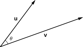
The GloVe algorithm is designed to produce similar vectors for semantically similar words. We can test how well the GloVe vectors capture semantic similarity with cosine similarity. In the figure below (source), vectors u and v are separated by an angle of θ:

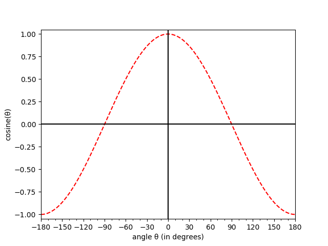
Two vectors that are separated by a small angle are more similar than two vectors separated by a large angle. Rather than find the actual angle in between the two vectors, we will find the cosine of the angle between the two vectors. Notice in the plot below that when the angle between two vectors is 0, the cosine of the angle between the two vectors is 1. As the angle between the two vectors increases, the cosine of the angle decreases. When the two vectors are as far apart as possible (180 degrees rotated from one another), the cosine of the angle between them is -1.

In order to compute the angle between two vectors, you can use the following formula: \( \displaystyle cos(u, v) = \frac{u \cdot v}{\lvert u \rvert \lvert v \rvert} \) where \( u \cdot v \) is the dot product between the two vectors, and \( \lvert u \rvert \) is the length of vector \( u \), which you can calculate by taking the square root of the sum of the squares of the elements in the vector: \( \lvert u \rvert = \sqrt{\sum_i u_i^2} \).

Don’t write any code for this just yet – read the next section first.

Computing lengths

If you only needed to compute the cosine similarity between two vectors, you could just use the formula above, taking the dot product and then dividing by their lengths. However, you’re going to be computing the cosine similarity between lots of vectors, lots of times, and calculating the length of the vectors over and over will make your program slower.

Good news! You don’t actually have to compute the square root of the sum of the squares in order to find the length of a vector: numpy will do this for you. The example below shows how to compute the length of a single vector i in the array:

vector = array[i]
vector_length = numpy.linalg.norm(vector)

Even better news! If you want to compute the norm (length) of a whole matrix, numpy can do that as well; you just have to tell it which direction (e.g. rows or columns for a 2-dimensional array like ours) you want it to find the length for. You can tell numpy to perform an operation row-wise on a 2-dimensional matrix by passing it the parameter axis=1:

array_lengths = numpy.linalg.norm(array, axis=1)

Write a function called compute_lengths in your utilities.py file that takes the array as its only parameter and returns a new array that stores the lengths of each row in the array. The array of lengths should have as many entries as there are rows in the large array.

Once we compute the vector lengths, we shouldn’t need to do it again, so modify your save_glove_vectors and load_glove_vectors function to also save the lengths to the .npy file.

• In your save_glove_vectors function, leave the arguments the same. In order to save the array of vector lengths to the .npy file, just call compute_lengths from within the save_glove_vectors function and then save them.
• In your load_glove_vectors function, you will now need to return a 3-element tuple that include the list of words, the array, and the array of vector lengths.
• Update any code you’ve written so far that calls load_glove_vectors to be sure you can handle the new return value.

Computing the cosine similarity

Now that you have the lengths saved in an array, write a function called cosine_similarity in your cosine.py file that takes four parameters: two vectors and their corresponding lengths. Remember that to compute the cosine between two vectors you first compute their dot product and then divide by their lengths. You’ve already computed their lengths. You could compute the dot product by hand, but just like with computing their lengths, numpy has this code already built-in:

dot_product = numpy.dot(vector_1, vector_2)
similarity = dot_product / (length_1 * length_2)

Given a word, find the row number in the array

You’re ready to find the cosine similarity between the vector for cat and the vector for dog. Wait– which vectors are those? You’ll have to do something like this to get a vector for a particular word.

cat_index = wordlist.index('cat')
cat_vector = array[cat_index]
cat_length = lengths[cat_index]

If you find this syntax tedious, you’re welcome to add a function (in your utilities.py file) that takes a word, the wordlist, the array and the list of lengths, and returns the appropriate vector and its length. For example:

(cat_vector, cat_length) = get_vec('cat', wordlist, array, lengths)

Testing

One issue you might be having at this point is knowing if things are working correctly. Here are three tests that you can do to see if things are working well. The precision of your answers may be different depending on how you printed them out – that’s fine.

1. The index of the word cat in the list of words should be 5450.
2. The length of the vector for dog is 4.858045696798486.
3. The cosine similarity between the vector for cat and the vector for dog is 0.9218005273769252

Finding the top n closest vectors

Now that we can find the cosine between two vectors, write a function called closest_vectors that takes six parameters: a vector v, that vector’s length length, the list of words words, the array array, the list of vector lengths lengths, and an integer n.

For each vector in the array, compute the cosine similarity between v and every other vector in the array. Return a list of tuples containing the words that were closest along with their similarity. For example, if v1 was the vector for the word 'cat' and norm1 was the length of v1:

closest_vectors(v1, norm1, words, array, lengths, 3)
[('cat', 1.0000000000000004), ('dog', 0.9218005273769252), ('rabbit', 0.8487821210209759)]

Unsurprisingly, the vector for the word cat was closest since it is the same as the vector v1 that we passed in, so the angle was 0 and the cosine similarity was 1 – well, sort of. Floating point arithmetic is not exact, so when we found the dot product and divided by the length, we actually got just a tiny tiny bit more than 1. That’s fine! It’s not worth worrying about.

For the questions immediately below, just ignore the first result which will always be the original word with similarity 1.0, or just about 1.0. (Later we will care what this first result is, so don’t just throw away the first result!)

Running from the command line

When you run your cosine.py program from the command line, it should have the following interface:

usage: cosine.py [-h] [--word WORD] [--file FILE] [--num NUM] npyFILE

Find the n closest words to a given word (if specified) or to all of the words
in a text file (if specified). If neither is specified, compute nothing.

positional arguments:
  npyFILE               an .npy file to read the saved numpy data from

optional arguments:
  -h, --help            show this help message and exit
  --word WORD, -w WORD  a single word
  --file FILE, -f FILE  a text file with one-word-per-line
  --num NUM, -n NUM     find the top n most similar words (default 5)

If you want to find the 3 closest words to the word cat, you would write:

python3 cosine.py glove.6B.50d.npy --word cat -n 3

If you had a text file that had words (one per line) that you wanted to find the 5 closest for each of them (like, say, you were answering the question below and you put all of those words in a file), you could write:

python3 cosine.py glove.6B.50d.npy --file words.txt

Questions (Part 1)

1. For each of the following words, report the top 5 most similar words, along with the similarity. In your writeup, skip the result showing each word’s similarity to itself (which means you are really only going to report the 4 most similar words).
   1. red
   2. magenta
   3. flower
   4. plant
   5. two
   6. thousand
   7. one
   8. jupiter
   9. mercury
   10. oberlin

2. Discuss results that you find interesting or surprising. Are there any results you aren’t sure about?

3. Choose another 10 (or more) words and report your results. Did you find anything interesting? Share any/all observations you have made.

Plotting the vectors for related words

Store the solutions you write for this section (plotting vectors) to a file called visualize.py. You will want to import your code from the utilities.py into this file so that you can once again load the array of vectors and their associated words from the .npy file.

On the glove website, the authors report some images that show consistent spatial patterns between pairs of words that have some underlying semantic relationship. For example, the authors include this image which shows how pairs of words normally associated as (male, female) pairs are related spatially:

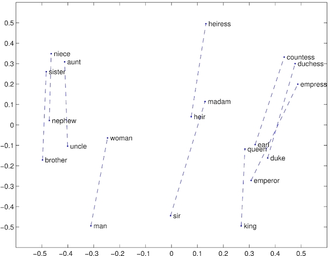
For this part of the assignment, we will try to duplicate their experiments. Given the GloVe vectors and a set of words with some semantic relationship, e.g. (male, female) nouns, we will plot the vector for each word and draw line connecting the two.

Plotting a multidimensional GloVe vector

We’d like to be able take a bunch of GloVe vectors and make a 2D plot. You’ll notice that our GloVe vectors are anywhere from 50 to 300 dimensions long, so we can’t just plot that directly. Instead, we will use principal component analysis (PCA) to reduce the dimensionality of the vectors down to 2. You don’t need to fully grasp how PCA works, and you’d need a course in Linear Algebra first, but reading through this short introduction to PCA might be helpful.

Extracting the words

We’re going to use scikit-learn, a Python machine learning library, to perform PCA for us. We don’t want to perform PCA on the whole array, though. Rather, we’re going to extract all the words in the pairs of related words that we’re interested in and put them into a new, smaller array. Then we’ll perform PCA on that.

Let’s assume you’ve somehow acquired a list of related words that you’d like to plot. For example:

related = [('brother', 'sister'), ('nephew', 'niece'), ('werewolf', 'werewoman')]

You want to go through the array and extract all the rows that match the words you want to plot. However, you only want to extract the rows if both words can be found in the array. For example, in the glove.6B.50d.txt file, the words ‘brother’, ‘sister’, ‘nephew’, ‘niece’, and ‘werewolf’ appear, but ‘werewoman’ doesn’t appear. You’ll want to extract the vectors only for ‘brother’, ‘sister’, ‘nephew’, and ‘niece’, skipping ‘werewolf’ (even though it has a vector) and ‘werewoman’.

Write a function called extract_words that takes three parameters: the array and wordlist that you read in from the .npy file, along with a list of related pairs. Your function will create a new numpy array that contains only the vectors for the pairs of words you are extracting. Your function will also create a new shorter list of words that align with the vectors in your new array. Return a tuple containing the new shorter list of words and the new smaller array. (Don’t worry about computing the vector lengths – you won’t need them for this part of the lab.)

NOTE: You will make your life a lot easier if you can extract the words into this new array in the order they appeared in the list of related words. This way, each even-indexed array row is followed by its corresponding pair. In this case, row 0 would be ‘brother’, followed by row 1 which would be ‘sister’; row 2 would be ‘nephew’, followed by and row 3 which would be ‘niece’.

Performing PCA

We will use the scikit-learn PCA class to perform PCA on our array of extracted vectors. Below is the code needed to perform PCA on your array:

from sklearn.decomposition import PCA  # put this at the top of your program

def perform_pca(array, n_components):
    # For the purposes of this lab, n_components will always be 2.
    pca = PCA(n_components=n_components)
    pc = pca.fit_transform(array)
    return pc

pca_array = perform_pca(array, 2)

Plotting the vectors

In this description, assume that the array you perfomed PCA on is called pca_array and the short list of words associated with that array is called pca_words.

This section will explain how to write a function you should call plot_relations. The function will take your pca_array and pca_words as parameters and will plot the vectors. There is no return value.

Let’s go ahead and directly plot all of the vectors in the array we just performed PCA on since they are all 2D vectors. In the example below, there’s the optional argument c which sets the color to r (red) and the optional argument s which sets the size of the point. You may wish to read the documentation for the matplotlib function scatter.

from matplotlib import pyplot as plt # put at the top of your file

fig = plt.figure(figsize = (8,8))
ax = fig.add_subplot(1,1,1)
ax.scatter(pca_array[:,0], pca_array[:,1], c='r', s=50)
plt.show()

(If you are using Docker, see the note at the bottom of the page.)

Assuming you used the short list of relations from above that included only ‘brother’, ‘sister’, ‘nephew’, and ‘niece’, you’d get this picture:

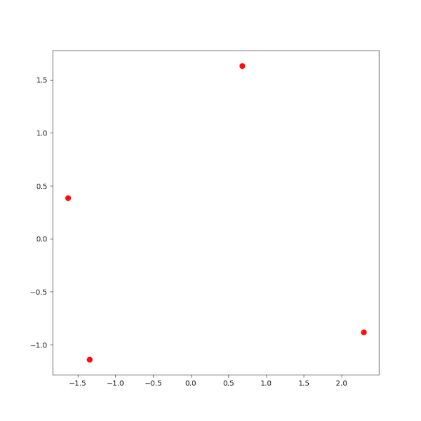
(After showing the plot, press the letter 'q' on the plot and it will close.)

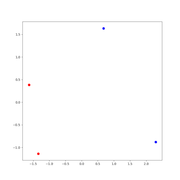
Coloring the points

We can improve on this picture by making the first half of the each relation in one color and the second half of each relation in another color. To do this, make two new lists of integers. In the first list of integers, store the row number where you will find all of the words that appear first in your relations (in this case, ‘brother’ and ‘nephew’). In the second list of integers, store the row number where you will find all of the second words (in this case, ‘sister’ and ‘niece’). Now try re-plotting as follows:

fig = plt.figure(figsize = (8,8))
ax = fig.add_subplot(1,1,1)
ax.scatter(pca_array[:,0][first], pca_array[:,1][first], c='r', s=50)
ax.scatter(pca_array[:,0][second], pca_array[:,1][second], c='b', s=50)
plt.show()

Now your picture should look like this, with ‘brother’ and ‘nephew’ in red, and ‘sister’ and ‘niece’ in blue.

Adding text labels

Now we’re getting somewhere! Two more important pieces to add. First, let’s add text labels to each of the dots so we know what each one is representing. This is a bit trickier to do in matplotlib, but basic idea is to iterate over each of the elements of the pca_array and annotate that (x,y) coordinate with the associated word:

for i in range(len(pca_array)):
  (x,y) = pca_array[i]
  plt.annotate(pca_words[i], xy=(x,y), color="black")

Put that code before the plt.show() line in the example above and you should get text labels attached to your data points.

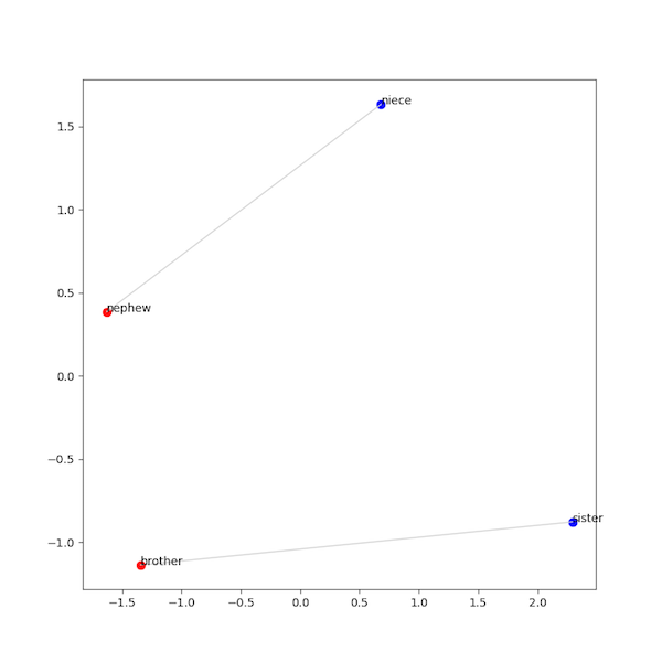
Connecting pairs of related words

Finally, let’s connect pairs of related words with a line. If you followed the note above about extracting the related words in the same order as you found the words in the relations, all you need to do now is make a vector that connects each even-indexed element in the pca_array with the following odd-indexed element:

for i in range(0, len(pca_array), 2):
    ax.plot(pca_array[:,0][i:i+2], pca_array[:,1][i:i+2],
    linewidth=1, color="lightgray")

If you add that code before the plt.show() you should now have a picture that looks like this:

Putting it all together

Write a function called read_relations that takes a file pointer as its only parameter, reads the relations, and stores them in a list of tuples as shown above. In the /data/glove/relations/ directory there are some files that contains pairs of relations. Each file starts with a header and then is followed by the pairs of words. For example, here is the start of the gender.txt file:

male    female
brother sister
nephew  niece
uncle   aunt

Now you should be able to:

1. Read in the array and words from a saved .npy file using the load_glove_array function in your utilities.py file,
2. Read in the list of relations using read_relations,
3. Extract the vectors you want to plot using extract_words,
4. Perform PCA on the these vectors using perform_pca, and finally
5. Plot these vectors using plot_relations

Running from the command line

When you run your visualize.py program from the command line, it should have the following interface:

$ python3 visualize.py --help
usage: visualize.py [-h] npyFILE relationsFILE

Plot the relationship between the GloVe vectors for pairs of related words.

positional arguments:
  npyFILE        an .npy file to read the saved numpy data from
  relationsFILE  a file containing pairs of relations

optional arguments:
  -h, --help     show this help message and exit

For example, to run on the capitals.txt file found in /data/glove/relations, you would write:

python3 visualize.py glove.6B.50d.npy /data/glove/relations/capitals.txt 

Questions (Part 2)

1. Plot each of the relations found in the /data/glove/relations/ directory. What did you find? Did the plots look like you expected them to look? Were there any anomalous data points? Which ones? Can you explain why?
2. Make your own relations files with ideas that you have about words you think might follow a similar pattern to the ones you’ve seen. You decide how many words are in the file and what the words are. Save the images of the plots you make and include them in your writeup. (Check the Markdown Cheatsheet to see how to include images in your markdown file.)
   1. Answer the same kinds of questions you did before, e.g. What did you find? Is it what you expected? etc.
   2. Repeat for as many as you’d like, but at least 2 different sets of relations files would help you see if there are patterns.

Just pretty pictures?

You might be impressed by some of the plots you made. These plots illustrate that some pairs of words seem to have a consistent relationship between them that you can visualize as a new vector connecting the two data points.

A question you might be asking at this point is: do these connecting vectors have predictive power? That is, if you found the vector that connected ‘France’ to ‘Paris’, could you use that information to figure out what the capital of ‘Hungary’ was?

Make a new file called predict.py. You’ll want to import utilities.py, cosine.py and visualize.py code in order to minimize the amount of additional code you need to write.

Average vector difference

Let’s say we have two vectors, a and b, that correspond to two words in our relations file, say, ‘paris’ and ‘france’. Using the array of vectors you read from the .npy file, we can subtract the vectors to find the vector that connects them (source):

To perform vector subtraction is straightforward since our data is in a numpy array: we can just subtract them.

# assume i is the index for 'paris'; j is the index for 'france'
a = array[i]   
b = array[j]
difference = a - b

If we compute this difference for all the pairs in a single relations file, we can then find the average vector that connects the second word in a relation back to the first word. You can visualize the average vector as follows (source):

Computing an average of vectors in numpy is straightforward: add them all up and then divide by the number of vectors you averaged.

# assuming vec_lst is a list of vectors to average
vec_average = sum(vec_lst) / len(vec_lst)

Write a function called average_difference that takes your original array (not your PCA array), your list of words, and your list of relations, and returns the average vector that connects the second word to the first word. Before trying to find the average, you’ll want to call your extract_words function (from visualize.py) to be sure you are only including vectors when both pairs in a relation are present in the GloVe vectors.

Predictive ability

Earlier in the lab you wrote code that found the most similar word to words like ‘red’ and ‘jupiter’. In this final part of the lab, we’re going to see if we can use the average vector above to make predictions about how words are related.

Repeat each of the questions below with each of the relations files provided in the /data/glove/relations/ directory. You’ll need to have read in the array and words from the .npy file as well as a list of relations from the relations file. (Hint: it might be good if you wrote an argparse interface to this, right?)

Before you begin to answer the questions, perform the following steps:

1. Given a list of relations, shuffle the list so that the order that they appear in the list is randomized. Pairs of words should remain together!
2. Create a list called training_relations that contains the first 80% of the relations in this shuffled list. (Round, as necessary, if your list isn’t evenly divisible).
3. Create a list called test_relations that contains the last 20% of the relations in this shuffled list. Your training_relations and test_relations lists should not contain any overlapping pairs and, between them, should contain all of the original relations.
4. Using your average_difference function, find the average difference between all of the words in your training_relations.

Questions (Part 3)

1. For each vector representing the second word in the test_relations, use your closest_vectors function to find the 100 most similar vectors/words. Exclude the first result since it will be the original word.
   1. How often is the first word in the relation also the most similar word?
   2. How often is the first word in the relation in the top 10 most similar words?
   3. Report the average position you found the first word in the results. If the word was not in the top 100, use 100 as its position so that you can find the average across all words.
2. For each vector representing the second word in the test_relations, add the average vector difference you computed above to this vector. This will make a new vector whose length you do not know, so you’ll have to call numpy.linalg.norm on it to find its length. Now you can use your closest_vectors function to find the 100 most similar vectors/words to this new vector (and its new length). The first result may not be the original word any more so don’t throw it away!
   1. How often is the first word in the relation also the most similar word?
   2. How often is the first word in the relation in the top 10 most similar words?
   3. Report the average position you found the first word in the results. If the word was not in the top 100, use 100 as its position so that you can find the average across all words.
3. What did you just do? Explain in your own words what these two questions accomplished, if anything. Are you surprised at the results? Unsurprised?
4. OPTIONAL: You should probably repeat this experiment a couple times because you shuffled the data and so there was some randomness in the results you got.
5. OPTIONAL: You might want to repeat this experiment for the relations files that you created to see how this technique works on those.
6. OPTIONAL: Experiment! Are there other ideas/techniques that you want to try?
7. OPTIONAL: You used /data/glove/glove.6B/glove.6B.50d.txt for all of your experiments. You will get better results if you use the any of the following. Note that the further down the list you go, the longer it will take to load and save your vectors and, once you move on to the 42B file, it will take much longer to run the closest_vectors function.
   1. /data/glove/glove.6B/glove.6B.100d.txt
   2. /data/glove/glove.6B/glove.6B.200d.txt
   3. /data/glove/glove.6B/glove.6B.300d.txt
   4. /data/glove/glove.42B/glove.42B.300d.txt
   5. /data/glove/glove.840B/glove.840B.300d.txt – note that this set of GloVe vectors distinguishes between upper- and lower-case words so you may need to rewrite some of your relations if you plan on using these

Appendix: Docker notes

This section is only relevant to you if you are using Docker.

The matplotlib examples above expect that you can show your plot directly on the screen. If you don’t have an X server on your machine and/or you don’t have X forwarding set up, the plt.show() function will not work properly. Instead, you can have matplotlib save your plots directly to .png files. To do so, you’ll want to import matplotlib as follows:

import matplotlib
matplotlib.use('Agg')
import matplotlib.pylab as plt

Then, in your code where the example includes plt.show(), you can replace that with plt.savefig.

plt.savefig("plot.png")  # this is any filename

There are many optional parameters to savefig that you may wish to investigate by reading the documentation.