Python3
In this class, we’re going to using Python 3 and not Python 2. Depending on when you took intro CS, it’s possible you only know Python 2.
For the purposes of this class, you will find that there are two big hurdles you will face in transitioning from Python 2 and Python 3:
- You will type
python3at the command line. Typingpythonwill run Python 2. - In Python 3,
printis a function. This means that the syntax of print statements now requires that you use parenthesis just as you would for any other function.
#python 2
print "Hello, World."
print                       # just print an empty line
print "Put a comma to prevent",
print "going to the next line"

#python 3
print("Hello, World.")
print()                     # just print an empty line
print("Add a parameter to prevent", end=' ')
print("Going to the next line")
Docker
Over the course of the semester, many labs will require the use of external software libraries. Rather than figuring out how to install all of the libraries on your own computers, there is a Docker container that you can download. The container will contain all of code and libraries that you need for the semester. The container will be hosted on Docker cloud, so if there is a need to update the container, you will be able to easily pull the newest version from the cloud.
To get started, you will need to visit the Get Started with Docker page to download Docker Community Edition. You will need to login or create a free account Docker before you can download the software. After you’ve downloaded the software, follow the instructions to install it.
When your container is running, you will need to mount one of your local folders so that you can read/write files. Since you’ll be pulling git repos to your computer in order to complete the labs, it is a good idea to make a folder on your computer as the parent directory to hold each of the lab repos. Many labs will also have data (usually text corpora) that you will need to have access to in order to complete the lab. For the purposes of this example, let’s assume that I’ve set up the following on my Mac:
- Top-level folder to hold my repos:
/Users/richardw/Documents/nlp/ - Folder to hold data needed to complete the labs:
/Users/richardw/Documents/nlp/data/
To run docker, use the following command (wrapped on to two lines for readability, but you should type this as a single line):
docker run -it -h docker -v /Users/richardw/Documents/nlp:/nlp
   -v /Users/richardw/Documents/nlp/data:/data jmedero/nlp:fall2018 bash
If I was using Windows, I might have the following:
- Top-level folder to hold my repos:
C:\Users\richardw\My Documents\nlp - Folder to hold data needed to complete the labs:
C:\Users\richardw\My Documents\nlp\data
Notice that in the command below, even though the directory is called “My Documents”, Windows allows you to just call the folder “Documents” at the command line to avoid problems with spaces. Also notice that Windows allows you to use ‘normal’ Linux forward-slashes to specify the path (wrapped on to two lines for readability, but you should type this as a single line):
docker run -it -h docker -v C:/Users/richardw/Documents/nlp:/nlp
    -v C:/Users/richardw/Documents/nlp/data:/data jmedero/nlp:fall2018 bash
You’re welcome to change the location of your top-level folder and your data folder to anywhere you want on your computer, but leave the part after the colon (/nlp and /data) the same.
Although the container has both emacs and vi installed, you will probably find that using a more modern editor installed locally on your machine is easier to use. Since you’re editing files that are local to your computer, a local editor (e.g. atom or Visual Studio Code) is likely a better choice.
If your installation does not go smoothly or you have additional questions, please let me know.
Warmups
Put all of your code in a single Python file called tokenizer.py
and demonstrate that your functions work by writing a main function.
The answers to each of the questions in the lab writeup should be placed in a
markdown file called Writeup.md. Read about markdown syntax. You will probably want to use atom or Visual Studio Code to edit your markdown files since there is a built-in markdown previewer built into both of these editors.
You should call your main function using the following pattern which
will allow you to import this file in Part 2 of the lab.
if __name__ == '__main__':
    main()
The main function should be the only place where you print anything.
Part 1(a)
Write a function called get_words that takes a string s as its only argument. The function should return a list of the words in the same order as they appeared in s. Note that in this question a “word” is defined as a “space-separated item”. For example:
>>> get_words('The cat in the hat ate the rat in the vat')
['The', 'cat', 'in', 'the', 'hat', 'ate', 'the', 'rat', 'in', 'the', 'vat']
Hint: If you don’t know how to approach this problem, read about str.split() .
Part 1(b)
Write a function called count_words that takes a list of words as its only argument and returns a dictionary that maps a word to the frequency that it occurred in s. Use the output of the get_words function as the input to this function.
>>> s = 'The cat in the hat ate the rat in the vat'
>>> words = get_words(s)
>>> count_words(words)
{'The': 1, 'cat': 1, 'in': 2, 'the': 3, 'hat': 1, 'ate': 1, 'rat': 1, 'vat': 1}
Notice that this is somewhat unsatisfying because the is counted separately from The. We can easily fix this by lower-casing all of the words before counting them using str.lower:
>>> words = get_words(s.lower())
>>> count_words(words)
{'the': 4, 'cat': 1, 'in': 2, 'hat': 1, 'ate': 1, 'rat': 1, 'vat': 1}
Hints
-
If you don’t have experience using dictionaries, read about Python’s
dictdata structure. -
If you have experience using Python dictionaries, try using
collections.defaultdict, an advanced kind of dictionary that can simplify your code.
Be sure that you are confident in your ability to use dictionaries in Python as you’ll be using them a lot in this class. If you are confident about dictionaries, try to reimplement your solution using collections.Counter. (If you aren’t confident yet, come back and try this later!)
Part 1(c)
Write a function called words_by_frequency that takes a list of words as its only argument. The function should return a list of (word, count) tuples sorted by count such that the first item in the list is the most frequent item. The order of items with the same frequency does not matter (but you could try to sort such items alphabetically if you were so inclined).
>>> words_by_frequency(words)
[('the', 4), ('in', 2), ('cat', 1), ('hat', 1), ('ate', 1), ('rat', 1), ('vat', 1)]
Hint: To sort a list of tuples by the second field, use the operator.itemgetter function:
  >>> import operator
  >>> tupleList = [('cat', 9), ('hat', 5), ('rat', 12)]
  >>> tupleList.sort(key=operator.itemgetter(1), reverse=True)
  >>> tupleList
  [('rat', 12), ('cat', 9), ('hat', 5)]
Tokenization
In this part of the lab, you will explore some files from Project Gutenberg and improve on the code you just wrote by adding to and/or modifying the tokenizer.py program you began in the previous section.
Part 2(a)
In the /data/gutenberg/ directory there are a number of .txt files containing texts found in the Project Gutenberg collection. Read in Lewis Carroll’s “Alice’s Adventures in Wonderland”, which is stored in the file /data/gutenberg/carroll-alice.txt. Use your words_by_frequency and count_words functions from Part 1 to explore the text. Assuming that you wrote your code properly in Part 1, and assuming that you lower-cased all of the words in the text, you should find that the five most frequent words in the text are:
the      1603
and       766
to        706
a         614
she       518
Questions
-
Use your
count_wordsfunction to find out how many times the wordaliceoccurs in the text. -
The word
aliceactually appears 398 times in the text, though this is not the answer you got for the previous question. Why? Examine the data to see if you can figure it out before continuing.
Part 2(b)
We now see that there is a deficiency in how we implemented the get_words function. When we are counting words, we probably don’t care whether the word was adjacent to a punctuation mark. For example, the word hatter appears in the text 57 times, but if we queried the count_words dictionary, we would see it only appeared 24 times. However, it also appeared numerous times adjacent to a punctuation mark so those instances got counted separately:
>>> word_freq = words_by_frequency(words)
>>> for (word, freq) in word_freq:
...     if 'hatter' in word:
...         print('%-10s %3d' % (word, freq))
...
hatter      24
hatter.     13
hatter,     10
hatter:      6
hatters      1
hatter's     1
hatter;      1
hatter.'     1
Our get_words function would be better if it separated punctuation from words. We can accomplish this by using the re.split function. (We will talk more about regular expressions in class.) Be sure to import re at the top of your file to make re.split() work. Below is a small example that demonstrates how str.split works on a small text and compares it to using re.split:
>>> text = '"Oh no, no," said the little Fly, "to ask me is in vain."'
>>> text.split()
['"Oh', 'no,', 'no,"', 'said', 'the', 'little', 'Fly,', '"to', 'ask', 'me', 'is',
 'in', 'vain."']
>>> re.split(r'(\W)', text)
['', '"', 'Oh', ' ', 'no', ',', '', ' ', 'no', ',', '', '"', '', ' ', 'said', ' ', 'the',
 ' ', 'little', ' ', 'Fly', ',', '', ' ', '', '"', 'to', ' ', 'ask', ' ', 'me', ' ', 'is',
 ' ', 'in', ' ', 'vain', '.', '', '"', '']
Note that this is not exactly what we want, but it is a lot closer. In the resulting list, we find empty strings and spaces, but we have also successfully separated the punctuation from the words. Using the above example as a guide, write and test a function called tokenize that takes a string as an input and returns a list of words and punctuation, but not extraneous spaces and empty strings. You don’t need to modify the re.split() line: just process the resulting list to remove spaces and empty strings.
>>> tokenize(text.lower())
['"', 'oh', 'no', ',', 'no', ',', '"', 'said', 'the', 'little',
 'fly', ',', '"', 'to', 'ask', 'me', 'is', 'in', 'vain', '.', '"']
>>> print(' '.join(tokenize(text.lower())))
" oh no , no , " said the little fly , " to ask me is in vain . "
Part 2(c)
Use your tokenize function in conjunction with your count_words function to list the top 5 most frequent words in carroll-alice.txt. You should get this:
'        2871      <-- single quote
,        2418      <-- comma
the      1642
.         988      <-- period
and       872
Part 2(d)
Write a function called filter_nonwords that takes a list of strings as input and returns a new list of strings that excludes anything that isn’t entirely alphabetic. Use the str.isalpha() method to determine is a string is comprised of only alphabetic characters.
>>> text = '"Oh no, no," said the little Fly, "to ask me is in vain."'
>>> tokens = tokenize(text)
>>> filter_nonwords(tokens)
['Oh', 'no', 'no', 'said', 'the', 'little', 'Fly', 'to', 'ask', 'me',
 'is', 'in', 'vain']
Use this function to list the top 5 most frequent words in carroll-alice.txt:
the      1642
and       872
to        729
a         632
it        595
Part 2(e)
Iterate through all of the files in the /data/gutenberg/ directory and print out the top 5 words for each. To get a list of all the files in a directory, use the os.listdir function:
>>> import os
>>> directory = '/data/gutenberg/'
>>> files = os.listdir(directory)
>>> files
['austen-emma.txt', 'austen-persuasion.txt', 'austen-sense.txt', 'bible-kjv.txt',
 'blake-poems.txt', 'bryant-stories.txt', 'burgess-busterbrown.txt',
 'carroll-alice.txt', 'chesterton-ball.txt', 'chesterton-brown.txt',
 'chesterton-thursday.txt', 'edgeworth-parents.txt', 'melville-moby_dick.txt',
 'milton-paradise.txt', 'README', 'shakespeare-caesar.txt',
 'shakespeare-hamlet.txt', 'shakespeare-macbeth.txt', 'whitman-leaves.txt']
>>> infile = open(os.path.join(directory, files[0]), 'r', encoding='latin1')
This example also uses the function os.path.join that you might want to read about.
Note about encodings: This open function above uses the optional encoding argument to tell Python that the source file is encoded as latin1. We will talk more about encodings in class, but be sure to use this encoding flag to read the files in the Gutenberg corpus.
Questions
- Loop through all the files the
/data/gutenberg/directory that end in.txt. Is'the'always the most common word? If not, what are some other words that show up as the most frequent word? - If you don’t lowercase all the words before you count them, how does this result change, if at all?
Zipf’s law
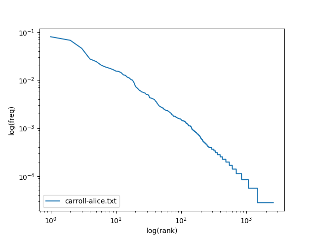
In this part of the lab, we will test Zipf’s law by using matplotlib, a 2D plotting library. Put your code for this part in a new file called zipf.py.
Part 3(a)
In this part of the lab, we will be exploring the relationship between the frequency of a token and the rank of that token. If you count all the tokens in carroll-alice.txt – like we did in Part 2(c) above – we would say that single quote has rank of 1, comma has rank of 2, the has a rank of 3, and so on, since this is the order that they appeared when we listed the tokens from most frequent to least frequent.
Be sure that you are using your tokenize function from above and
that you are not calling your filter_nonwords function but that you are
lowercasing the text. (If you don’t lowercase, the results will be slightly different, but you will reach the same conclusions.)
Let f be the relative frequency of the word (e.g. assuming you lowercased the text,
the occurs 1642 times out of 35652 tokens so its relative frequency is 1642/35652 =
0.04606) and r be the rank of that word.
To visualize the relationship between rank and frequency, we will
create a log-log
plot of rank (on
the x-axis) versus frequency (on the y-axis). We will use the pylab
library, part of matplotlib:
from matplotlib import pylab
from tokenizer import tokenize, words_by_frequency, count_words

text = open('/data/gutenberg/carroll-alice.txt', 'r', encoding='latin1').read()
words = tokenize(text.lower())
counts = words_by_frequency(words)
n = len(counts)
ranks = range(1, n+1)                     # x-axis: the ranks
freqs = [freq for (word, freq) in counts] # y-axis: the frequencies
pylab.loglog(ranks, freqs, label='alice') #this plots frequency, not relative frequency
pylab.xlabel('log(rank)')
pylab.ylabel('log(freq)')
pylab.legend(loc='lower left')
pylab.show()
Part 3(b)
Now we can test how well Zipf’s law works. Read Wikipedia’s article on Zipf’s law. In summary, Zipf’s law states that \(f \propto \frac{1}{r}\), or equivalently that \(f = \frac{k}{r}\) for some constant factor \(k\), where \(f\) is the frequency of the word and \(r\) is the rank of the word. Following Zipf’s law, the 50th most common word should occur with three times the frequency of the 150th most common word.
Plot the empirical rank vs frequency data (as we just did above) and also plot the expected values using Zipf’s law. For the constant \(k\) in the formulation of Zipf’s law above, you should use \(\frac{T}{H(n)}\) where \(T\) is the number of word tokens in the corpus, \(n\) is the number of word types in the corpus, and \(H(n)\) is the \(n^{th}\) harmonic number. The number of tokens is the total number of words in the document. The number of types is the total number of unique words in the corpus.
Use this function to compute harmonic numbers:
def H_approx(n):
    """
    Returns an approximate value of n-th harmonic number.
    http://en.wikipedia.org/wiki/Harmonic_number
    """
    # Euler-Mascheroni constant
    gamma = 0.57721566490153286060651209008240243104215933593992
    return gamma + math.log(n) + 0.5/n - 1./(12*n**2) + 1./(120*n**4)
To plot a second curve, simply add a second pylab.loglog(...) line immediately after the line
shown in the example above.
Questions
-
How well does Zipf’s law approximate the empirical data in
carroll-alice.txt? How many words (in total, not unique words - also called tokens) doescarroll-alice.txthave? -
Repeat the previous question for a few other texts included in the
/data/gutenberg/directory. - In your
tokenizer.pyfile, add a function calledall_files()that takes a directory as its only parameter and returns a string containing all of the.txtfiles in a that directory concatenated together. You should use code like you wrote in Part 2(e) to iterate through all of files in order to form one large string.- Use the
all_files()function to read in all of the texts and repeat the Zipf’s law experiment with this larger corpus. - How many tokens are in this new corpus?
- How does this plot compare with the plots from the smaller corpora?
- Use the
-
Does Zipf’s law hold for each of the plots your made? What intuitions have you formed?
- Generate random text, e.g., using
random.choice("abcdefg "), taking care to include the space character. You will need toimport randomfirst. Use the string concatenation operator to accumulate characters into a (very) long string. Then tokenize this string, and generate the Zipf plot as before, and compare the two plots. What do you make of Zipf’s Law in the light of this? (Source: Exercise 23b, Bird, Klein and Loper, 2009)
‘i’ before ‘e’ except after ‘c’
There is a commonly known rule in English that states that if you don’t know if a word is spelled with an ‘ie’ or an ‘ei’, that you should use ‘ie’ unless the previous letter is ‘c’. You can read about the ‘i’ before ‘e’ except after ‘c’ rule on Wikipedia if you haven’t heard of it before. Collecting statistics from text corpora can help us determine how good a ’rule’ it really is. We’ll begin by experimenting with the files in /data/gutenberg/ and use matplotlib
to make some graphs. Save your answers in ibeforee.py.
Part 4
In texts, many words will occur multiple times. For example, “soldiers” occurs 10 times in the carroll-alice.txt text. If I ask you to count types, then you should count unique words, and “soldiers”, despite occurring 10 times, would only count as 1 type. If I ask you to count tokens, then you should count each occurrence of
the word, so “soldiers” would be counted 10 times.
Read in all of the texts in /data/gutenberg/ into a single corpus like you did in Question (iv) in Part 3(b) above. Let’s call this combination of files the Gutenberg corpus.
Questions
-
Repeat these four parts for types and then for tokens using the Gutenberg corpus.
-
How frequent is ‘cie’ relative to all ‘ie’ words?
-
How frequent is ‘cei’ relative to all ‘ei’ words?
-
Compute the fraction of the words that contain ‘cei’ relative to all words that contain ‘cei’ or ‘cie’ by computing \(\frac{\texttt{count(cei)}}{\texttt{count(cie)+count(cei)}}\). This most directly answers the question “After a ‘c’, what’s more likely, ‘ie’ or ‘ei’?”
-
Is this answer what you expected or is it surprising?
-
-
The ‘i before e’ rule has some exceptions. Recompute your answers to the question above, but don’t count any word that has ‘eigh’, ‘ied’, ‘ier’, ‘ies’, or ‘iest’. How does this change your result?
-
Is ‘i before e except after c’ a good rule? Perhaps there’s a better rule, like “i before e except after h”? Repeat the previous question, substituting the letter ’c’ with all the possible letters. Report the relevant results and discuss.
Hint: To iterate through all possible letters, you can use code like this:
for letter in "abcdefghijklmnopqrstuvwxyz": print(letter) -
Experiment! Try something cool that I didn’t mention. This is optional, but it’s fun, so keep going! Or, for fun, try solving these questions using only bash scripting and feel free to use any scripting tools you know (e.g. perl, sed, awk, grep, wc, bc).