Use Teammaker to form your team. You can log in to that site to indicate your partner preference. Once the lab is released and you and your partner have specified each other, a GitHub repository will be created for your team.
The objectives of this lab are to:
You will implement the following local search methods:
You will need to modify the following python files:
You will not need to modify the following python files:
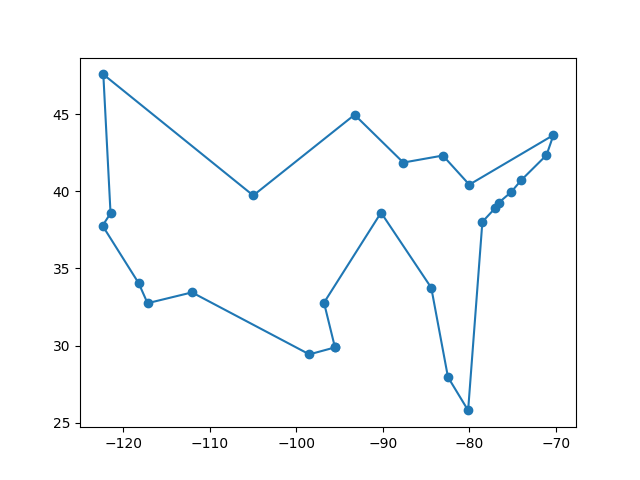
./LocalSearch.py HC coordinates/South_Africa_10.json
./LocalSearch.py SA coordinates/India_15.json
./LocalSearch.py BS coordinates/Lower_48.json
./LocalSearch.py SBS coordinates/Lower_48.json
The first example runs hill climbing to solve a TSP problem on the 10-city South Africa map. The second example runs simulated annealing to solve a TSP problem on the 15-city India map. The third and fourth example runs beam search and stochastic beam search on a TSP problem for a map of the lower 48 states in the United States.
NOTE: In order to execute python files directly (as shown above, without having to type python3), you'll need to make the file executable first. Type the following at the unix prompt to change the file's permissions:
chmod u+x LocalSearch.py
By default the best solution found will be saved to a file called map.pdf, and the parameters used for each search are defined in the file default_config.json. There are additional optional parameters you may add that allow you to load a non-default parameter file and/or save the resulting map to a non-default output file, e.g.:
./LocalSearch.py HC -config my_config.json -plot USA25_map.pdf
Local search is typically used on hard problems where informed search is not viable (for example TSP is an NP-complete problem). Thus the search often runs for an extended period of time. It is entirely normal for runs to take several seconds to complete on the larger maps; however, if you find your program running for multiple minutes then there's likely something incorrect, or inefficient, about your implementation. For reference, my implementation of Stochastic Beam Search takes around 10 seconds on the 250 node map (you don't need to match this time, but it should give you a ballpark for what's possible).
It is therefore important to keep the user informed of the search's progress. Each of your local search methods (HC, SA, BS, SBS), should print informative messages during the search execution. For instance, you should inform the user whenever the best value found so far is updated along with the current search step at that point.
Work on implementing your solution following the steps listed below.
A traveling salesperson tour visits each of a collection of cities once before returning to the starting point; we will assume all cities are connected (i.e. the problem forms a complete graph). The objective is to minimize the total distance traveled (we will make the simplifying assumption that the graph is planar, meaning we just need to compute the Euclidean distance between the city locations). We will represent a tour by listing cities in the order visited. 'Neighbors' or 'successors' of a tour are produced by moving one city to a new position in the ordering.
The class TSP, defined in the file TSP.py, represents instances of the traveling salesperson problem. Here are some useful methods within this class:
Instances of the TSP class are constructed by passing in the name of a JSON file specifying the latitude and longitude of locations that must be visited. Example JSON files are located in the coordinates directory.
Note that the TSP method _all_neighbors() begins with a single underscore. This is a python convention for indicating a 'private' method. Python doesn't actually distinguish between private and public class members, but the underscore lets programmers know that the method isn't intended to be called directly. In this case, your local search functions should not call this method. However, other methods within the class definition may call such private methods.
You should incrementally test your code as you develop it. The best way to do this is to add tests inside the if at the bottom of the TSP.py file:
  if __name__ == '__main__':
     ...
Once you have completed and tested the implementations in the TSP.py file you can move on to start implementing the local search methods.
candidate = problem.random_candidate()
cost = problem.cost(candidate)
return candidate, cost
This will allow you to run hill climbing without generating errors:
./LocalSearch.py HC coordinates/United_States_25.jsonDoing so will print the random candidate and its cost, and will also create a file that plots the tour in latitude/longitude coordinates. By default the plot is saved in a file called map.pdf.
Your next job is to implement the following hill climbing algorithm. This is a slightly different version than what we discussed in class. With some probability (determined by one of the parameters) it will take a random move. It will always execute the requested number of steps (rather than terminating when it reaches a local maximum), keeping track of the best state found so far. The entire search will be repeated the requested number of times, and the best candidate found in any of the runs will be reported as the solution found.
initialize best_state, best_cost
loop over runs
  curr_state = random candidate
  curr_cost = cost(curr_state)
  loop over steps
    if random move
      curr_state, curr_cost = random neighbor of curr_state
    else
      neighbor_state, neighbor_cost =  best neighbor of curr_state
      if neighbor_cost < curr_cost:
         update curr_state, curr_cost
    if curr_cost < best_cost
       update best_state, best_cost
       print status information about new best cost
return best_state, best_cost
Note that computing the cost of a tour takes non-trivial time, so whenever
possible, you should store the value rather than making another function
call. This doesn't mean you need to create some sort of global cache of
pre-computed values, since that would take way too much memory, but it
does mean you shouldn't generate the cost of the same path multiple
times during a single loop iteration.
Several of the parameters used above are specified in a config file. By default, LocalSearch.py reads default_config.json. You may want to copy this file and modify it:
cp default_config.json my_config.jsonThen edit the "HC" portion of my_config.json to whatever defaults you would like to use. Then you can re-run the local search based on your own selections rather than the default ones.
./LocalSearch.py HC coordinates/South_Africa_10.json -config my_config.json
Remember that if typing long commands gets tedious, you can use the up-arrow key in the terminal to scroll through previously executed commands. You can also type long commands, or even sequences of commands, into a shell script that you can run later.
Once your hill climbing search is successfully finding good tours for the easier problems with fewer cities, you can move on to the next local search algorithm.
SimulatedAnnealing.py is set up much like HillClimbing.py. Your next task is to implement the algorithm that we discussed in class. Here, our cooling schedule will use a exponential weighted decay; in other words, we'll multiply the current temperature by a fixed decay rate (which will be slightly less than one) after each step. We will use the 'slightly greedy' variant that always moves to a 'better' state and only checks the probability to decide whether to move to a 'worse' state.
initialize best_state, best_cost
loop over runs
  temp = init_temp
  curr_state = random starting state
  curr_cost = cost(curr_state)
  loop over steps
    neighbor_state, neighbor_cost = random neighbor of curr_state
    delta = curr_cost - neighbor_cost
    if delta > 0 or with probability e^(delta/temp)
       curr_state = neighbor_state
       curr_cost = neighbor_cost
    if curr_cost < best_cost # minimizing
       best_state = curr_state
       best_cost = curr_cost
       print status information about new best cost
    temp *= temp_decay
return best_state, best_cost
Edit the "SA" portion of the config file to set the defaults for simulated annealing. The init_temp specifies the starting temperature, and temp_decay gives the geometric rate at which the temperature decays. The runs and steps parameters have the same interpretation as in hill climbing: specifying how many random starting points simulated annealing should be run from, and how long each run should last.
Once your simulated annealing search is successfully finding good tours, you can move on to the next local search algorithm.
BeamSearch.py is set up similarly to the other local searchs, with the exception that you will implement two closly related algorithms together.
You will implement both the 'plain' and the 'stochastic' versions of the Beam Search algorithm; in this case, you will implement both algorithms in the same file, since there are significant overlaps and you'll want to avoid code replication by extracting the common functionality into helper functions.
Again, you can edit the "BS" and "SBS" portions of the config file to set the defaults for these searches.
Beam search performs multiple searches in parallel; however, instead of starting several separate runs like we did for Hill Climbing, beam search maintains a population of candidates at each step. The pop_size parameter specifies the number of candidates.
Your final implementation task is to implement the beam search algorithm as discussed in class:
initialize best_state, best_cost_so_far
pop = initial population of pop_size random states
loop over steps
  generate max_neighbors random successors of each member of pop
  find overall best_neigh_cost and associated best_neigh_state
  if best_neigh_cost < best_cost_so_far
     update best_cost_so_far, best_state
     print status information about new best cost
  pop = pop_size successors selected by picking the best ones
Beam Search generates neighbors of all the candidates in the population, puts them all together in one big bag, and then considers them uniformly (i.e. it doesn't care which member of the population generated which neighbor). It just keeps the best neighbors found to replace the previous population with a new one of the same size (i.e. the size of pop should always be pop_size)
Note that our implementation will generate max_neighbors successors for each element in pop. Some versions of this algorithm call for generating every possible neighbor of each element in pop, but we will not do this. There are several reasons for this choice, but the main ones are that it is very computationally expensive and that it encourages premature convergence.
For the larger maps, the number of neighbors grows quite large, making it impractical to evaluate every neighbor of every candidate. Your helper function should therefore consider only a random subset of each individual's neighbors. The size of this subset is given by the max_neighbors parameter in the "BS" and "SBS" sections of the config file.
Remember, you will want to use helper functions for common behaviors! Think about what steps Beam Search and Stochastic Beach Search have in common and turn them into helper functions during your design phase. Then, after implementing both of them, look at them and consider whether there remain significant blocks of replicated code that can be extracted and turned into helper functions.
Stochastic Beam Search uses a population of candidates at each step, but it also uses temperature and steps parameters similar to simulated annealing.
Your final implementation task is to implement the stochastic beam search as discussed in class:
initialize best_state, best_cost
pop = initial population of pop_size random states
temp = init_temp
loop over steps
  generate max_neighbors random successors of each member of pop
  find overall best_neigh_cost and associated best_neigh_state
  if best_neigh_cost < best_cost
     update best_cost_so_far, best_state
     print status information about new best cost
  generate probabilities for selecting neighbors based on cost
  pop = pop_size neighbors selected by random sampling w/ probs
  temp *= decay
Stochastic beam search considers neighbors of all individual candidates in the population and preserves each with probability proportional to its temperature score. It is recommended that you add a helper function that evaluates the cost of each neighbor and determines its temperature-based probability score, then randomly selects the neighbors that will appear in the next iteration according to the probabilities. Remember to avoid excess calls to cost by saving the value whenever possible.
A very useful python function for stochastic beam search is numpy.random.choice. This function takes a list of items to choose from, a number of samples to draw, and optionally another list representing a discrete probability distribution over the items. It returns a list of items that were selected. Here is an example:
import numpy.random
items = ["a", "b", "c", "d", "e"]
indices = list(range(len(items)))
probs = [0.1, 0.1, 0.2, 0.3, 0.3]
for i in range(5):
  choices = numpy.random.choice(indices, 10, p=probs)
  print(choices)
In this particular example, items "d" and "e" have the highest probability of being selected (30 percent chance each), and they are at indices 3 and 4. You can see in the sample results below that indices 3 and 4 are selected more often on average than indices 0, 1, and 2.
[3 2 2 2 4 3 4 4 4 4]
[3 4 2 4 4 4 4 4 4 3]
[4 4 4 3 4 2 3 0 3 2]
[4 2 3 0 1 0 3 4 4 2]
[4 0 1 4 4 2 4 0 4 3]
Unfortunately, numpy will treat a list of Tours as a multidimensional array, so it is better to select indices (as demonstrated above) rather than choosing from a list of neighbors directly.
Note that depending on the config values you start with, in the later stages of the search some of the probabilities may become very small, to the point that they may underflow the floating point representation and end up with a value of 0. If this happens, you're likely to run into math exceptions (e.g. divide by zero). There are a few options here, but the simplest to implement is to put the dangerous code in a try statement and handle the exception by simply concluding the search and returning the best candidate found so far.
Once your stochastic beam search is successfully finding good tours, you can move on to final step of comparing the four local search algorithms.
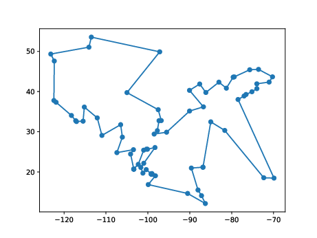
After all four of your local search algorithms are complete and working correctly, do some experimental comparisons between the algorithms on the coordinates North_America_75.json. Be sure to spend a little time trying to tune the parameters of each algorithm to achieve its best results. If you find any particularly impressive tours, save them by renaming the file map.pdf to a more informative name.
In the file called summary.md, fill in the tables provided with your results and explain which local search algorithm was most successful at solving TSP problems. Did the outcome match your hypothesis that you voted on in class?