Lab goals
- Use git to clone the repo for this lab
- Understand how to activate and deactivate the cs81 virtual environment
- Learn how to use Jupyter Notebooks
- Learn how to control a simulated robot in Jyro
- Program a simulated robot to find a light source
Introduction
In this class we will be investigating ways to make robots be more adaptive--to learn about themselves and their environment by exploring what they can achieve rather than being told how to behave. Because this learning process can be quite slow and physical robots have limited battery life, we will be focusing on simulated robots rather than physical robots. This week, we will begin by learning how to program simulated robots directly, without any learning. In subsequent labs we will add learning.
1. Using git
Log on to the github server. Then choose the CS81-f17 organization in the drop down menu under your username. Select the link for this lab, then press the Clone or Download button. Be sure that you have Clone with SSH selected. Copy the link provided. The go to a terminal window and make a directory for this class. Change into your directory and type:
git clone [link you copied]Change into the lab directory. Now you're ready to get started with the lab. Note: You only have to do this step once for each lab.
2. Virtual Environment
We have created a virtual environment that you will need to invoke each time you want to start working on the labs for this class. This environment includes python 3 (rather than python 2, which is the default on our system), the Jyro robot simulator, Jupyter Notebooks, and deep learning software (such as conx, keras, and tensorflow). In your terminal window type:
source /usr/swat/bin/CS81envYour terminal prompt should now have the prefix (cs81venv).
To exit the virtual environment type:
deactivateYour terminal prompt should return to normal. Try activating and deactivating this virtual environment at least once. Be sure to re-activate the environment before moving on.
3. Jupyter Notebooks
A notebook is a document that can contain both executable code and explanatory text. It is a great tool for documenting and illustrating scientific results. In fact, this lab writeup is a notebook that was saved as an html file. A notebook is made up of a sequence of cells. Each cell can be of a different type. The most common types are Code and Markdown. We will be using Code cells that are running Python 3, though there are many other possibilities. Markdown cells allow you to format rich text.
In your terminal window, where you are already in your cs81 lab directory and have activated the virtual environment, type the following to start a notebook:
jupyter notebookA web browser window will appear with the Jupyter home screen. On the right-hand side, go to the New drop down menu and select Python3. A blank notebook will appear with a single cell.
Let's try writing and executing a simple hello program. One of the main differences between Python 2 and Python 3, is that print is a function in Python 3. When you are ready to execute the cell, press Shift-Enter.
def hello(name):
    print("Hi", name)

hello("Chris")
hello("Samantha")
Now let's try creating a Markdown cell. In the tool bar of the notebook you'll see a drop down menu where you can choose the cell's type. By default, each cell will be a Code type. With your cursor in a new cell, select Markdown from this menu.
Check out this Markdown cheat sheet to see all of the text formatting options available in Markdown. Try to make a Markdown cell that looks like the one below. You need to execute Markdown cells using Shift-Enter just as you do with Code cells.
Things to do in the Science Center
- Get a smoothie at the Coffee Bar
- Visit the Computer Science Department
To name your notebook, double click on the default name, Untitled, at the top. Let's call it FirstNotebook. To save a notebook, click on the disk symbol on the left-hand side of the tool bar. You can also use the File menu and choose Save and Checkpoint. Explore the other menu options in the notebook. Figure out how to insert and delete cells, which are common commands you'll need to know.
To exit a notebook, save it first, then from the File menu choose Close and Halt. In the terminal window where you started the notebook, you'll also need to type CTRL-C to shutdown the kernel. Do an ls to list the contents of your directory. You'll see that you now have a file called FirstNotebook.ipynb.
Now that you know how to use a notebook, we can learn how to simulate a robot within a notebook.
4. Jyro Simulator
In a terminal window, where you are already in your cs81 lab directory and have activated the virtual environment:
- Start up jupyter notebook.
- Create a new Python 3 notebook.
- Name it JyroTest.
The first step is to import the Jyro simulator. Note: Try all of these code cells in your own notebook.
from jyro.simulator import *
To use the simulator, you need to define a world and a robot.
We will define a very simple world that is enclosed in a 4x4 box (the origin is at the bottom left corner). It contains a light source centered at the top, which is blocked by a small blue wall.
def make_world(physics):
    physics.addBox(0, 0, 4, 4, fill="backgroundgreen", wallcolor="gray") #bounding box
    physics.addBox(1.75, 2.9, 2.25, 3.0, fill="blue", wallcolor="blue")  #inner wall to hide the light behind
    physics.addLight(2, 3.5, 1.0) #paramters are x, y, brightness
We will be using a simulated Pioneer robot, which is based on the real, physical robot shown below.
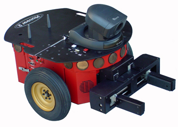
The pictured robot has a camera, sonars, and a gripper. We will define a simulated robot with a camera, sonars, and light sensors.
def make_robot():
    robot = Pioneer("Pioneer", 2, 1, 0) #paremeters are name, x, y, heading (in radians)
    robot.addDevice(Camera())
    robot.addDevice(Pioneer16Sonars())
    light_sensors = PioneerFrontLightSensors(3) #parameter defines max range in meters
    robot.addDevice(light_sensors)
    return robot
The robot has been positioned at the bottom, center of the world. Headings for robots are in the range [0.0, 2pi], where 0=north, pi/2=east, pi=south, and 3pi/4=west. Here we've positioned the robot at heading 0, which is north.
We can now create a visual simulator that allows us to manipulate the robot and see how it behaves in real time. Later in the semester, when we are running learning experiments, we will use a non-visual simulator that will execute much faster.
robot = make_robot()
vsim = VSimulator(robot, make_world)
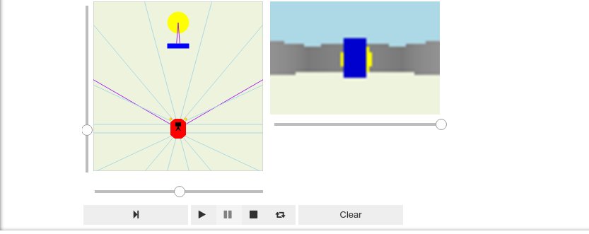
This will bring up the simulator in your notebook. It provides a top-down view of the world and the robot along with an image from the robot's camera. Try using the sliders to manipulate the robot's x, y, and heading. Note that the camera image changes based on the robot's new location. You can get the robot's current (x, y, heading) by using the getPose() method:
robot.getPose()
You can also place the robot in a particular position by using the setPose(x, y, heading) method. You'll have to also update the visual simulator to see the new location.
robot.setPose(1, 1, 3.14)
vsim.update_gui()
Light Sensors
The robot is equipped with two light sensors positioned on the front of the robot. These are depicted as small yellow circles on the left and right front of the robot. When a light sensor has a clear view of a light source, an orange line will emanate from the sensor to the source. When a light sensor is blocked, a purple line is drawn between the light source and the obstacle. These sensors return values in the range [0.0, 1.0], where 1.0 indicates a maximum light reading and 0.0 indicates no light sensed. Use the simulator's sliders to move the robot to different locations in the world and observe how the light sensor data changes.
robot["light"].getData()
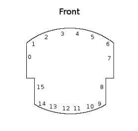
Sonar Sensors
The robot is equipped with 16 sonar sensors positioned around its perimeter (as shown below). These sensors return values in the range [0.0, maxRange], where maxRange depends on the size of the world. Each sonar measures the distance to an obstacle. Small values, close to 0.0, indicate that an obstacle is very near. Larger values indicate that there is open space at that angle relative to the robot. The blue lines emanating from the robot in the simulator represent its sonar sensors. Observe how these sonar readings vary as you move the robot around in the world.
robot["sonar"].getData()
Camera Sensor
The robot is equipped with a camera that is positioned on the front of the robot and is depected as a black rectangle on the simulated robot. The purple lines emanating from the robot show the camera's viewing range. The camera grabs images that are 60 x 40 pixels. The camera image is automatically displayed by the visual simulator, but you can also use the command given below to grab an image.
robot["camera"].getImage()

We'll learn more about the camera and the image representation in later labs.
Robot Movement
You control the robot's movement by telling it how fast to translate (either forward or backwards) and how fast to rotate (either right or left). The translation amount ranges from [-1.0, 1.0], where -1.0 indicates full backwards, and 1.0 indicates full forwards. The rotation amount ranges from [-1.0, 1.0], where -1.0 indicates full right rotation, and 1.0 indicates full left rotation.
Insert a cell just below the visual simulator in your notebook. In that cell try several different movement commands (such as those shown below), one at a time. Remember to execute the cell using Shift-Enter and then press the Play button on the simulator. The simulator will repeatedly execute the last move command given to the robot. Press the Stop button on the simulator and the robot will halt and return to the starting location.
robot.move(-1, 0) # straight back
robot.move(1, 0) # straight forward
robot.move(0.3, 0.3) # slow forward, left arc
robot.move(0, -1.0) # turning right in place
Stall Sensor
Every Jyro robot is automatically equipped with a stall sensor; you don't need to explicitly add this sensor when you define a robot. The stall sensor returns a 1.0 when the robot is trying to move, but it can't, otherwise it returns 0.0. It operates like a boolean flag indicating stuck or not stuck. Try to get the robot stuck by moving it toward a wall. Then test that the stall sensor returns 1.
robot.stall
Creating a Robot Brain
You can create a robot brain by defining a function that takes the robot as a parameter, checks the current sensor readings, and executes a single movement. The brain will be repeatedly called by the simulator to create continuous behavior. For example, suppose we wanted to create a brain that would simply wander around and avoid hitting any obstacle.
def avoidBrain(robot):
    sonars = robot["sonar"].getData()
    front = min(sonars[1:7])
    if front < 0.5:           # check for an obstacle
        robot.move(0.0, -1.0) # stop and turn right
    else:
        robot.move(1.0, 0)    # otherwise go straight

robot.brain = avoidBrain
When you press the Play button on the simulator, this brain will execute. When you press the Stop button, the brain will stop and the robot will return to the starting point.
Modify this brain so that it works differently. For example, you could avoid obstacles sooner, or you could turn left instead of right, or you could you choose which direction to turn based on which side of the robot is closer to the obstacle. After each change remember to execute the cell and then press the Play button to test the brain.
Once you are done exploring Jyro save your notebook. Now you are ready to write your own robot brain.
5. Find Light Brain
Open a new notebook called RobotFindLight. Then create a sequence of Code cells to do the following:
- Import any python libraries that you need, such as jyro.simulator.
- Define the same world that we've been using so far.
- Define a robot with just sonar and light sensors. You won't need a camera sensor.
- Make the robot and the simulator. You'll notice that the camera image section of the visual simulator will be blank, because there is no camera device on the robot.
- Create a brain that causes the robot to go to the light source. Starting from any location in the world, the robot should be able find the light source, while also avoiding obstacles. When the robot reaches the light, it should stop.
- Use Markdown cells to document your code.
You should use git to add, commit, and push the file RobotFindLight.ipynb. This file will be graded for this lab.