In this lab you will experiment with an evolutionary computation method called NEAT (Neuro Evolution of Augmenting Topologies) developed by Kenneth O. Stanley. NEAT operates on both the weights and the structure of a neural network, allowing connections and nodes to be added as potential mutations. You will be using the simulators you wrote last week combined with a python package that implements NEAT to evolve neural network controllers to produce motions that maximize coverage of the world.

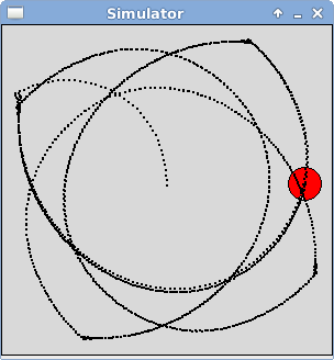
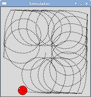
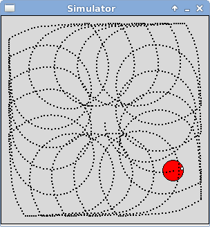
For example, the images above show the best performing networks from generation 0, 4, and 5 of one run of NEAT, using coverage as the fitness function. In generation 0 (on the left), the controller re-traces over the same paths again and again. In generation 4 (in the center), the controller makes smaller looping motions that are slightly shifted each time, managing to cover a larger percentage of the world. In generation 5 (on the right), the controller uses a similar technique as in the previous generation, but moves more efficiently in the same amount of time and is now covering an even larger portion of the world.

You will begin by verifying that your simulator is working correctly. Next you will add some features to your simulator to allow the robot to leave a trail of its locations, and to calculate coverage. Then you will experiment with NEAT, testing out different parameter settings and documenting your results.

If at any point you are interested in seeing the source code for the NEAT package, you can cd into the following directory on our system:

/usr/local/stow/cs81/lib/python2.6/site-packages/neat

Go through the following steps to setup your directory for this lab.

1. First you need to run setup81 to create a git repository for the lab.

   If you want to work alone do:

   setup81 labs/03 none

   If you want to work with a partner, then one of you needs to run the following while the other one waits until it finishes.

   setup81 labs/03 partnerUsername

   Once the script finishes, the other partner should run it on their account.

2. For the next step only one partner should copy over the starting point code. First you will copy over your simulator from last week and then you will copy over files from my public directory.

   cd ~/cs81/labs/03
   cp ../02/simulator.py .
   cp -r ~meeden/public/cs81/labs/03/* ./
   

3. Whether you are working alone or with a partner, you should now add all of the files to your git repo, commit, and push them as shown below.

   git add *
   git commit -m "lab3 start"
   git push
   

4. If you are working with a partner, your partner can now pull the changes in.

   cd ~/cs81/labs/03
   git pull
   

Before using your simulator to conduct evolutionary computation experiments, you need to verify that it is working properly. Let's run some basic tests to confirm this. Edit your simulator.py file in the labs/03 directory.

First you'll need to add some simple brains called ForwardBrain (returns 1, 0), BackwardBrain (returns -1, 0), RotateLeftBrain (returns 0, -1), RotateRightBrain (returns (0, 1) and CircleBrain (returns 1, 0.5).

Next you'll create a main program that confirms that all of these brains work properly. Your main program should set up the world and the agent as follows:

Create a world of size 300 by 300
Create an agent at the center of this world facing East with a radius
of 25, a translation speed of 15, and a rotation speed of 6
Make the agent visible and red in color
Add the agent to the world

Now test left rotation. Since the rotation speed is 6, it should take 60 steps for the agent to rotate one full time around (360 degrees). While the agent is turning, print it's current status so that you can confirm that the heading is being updated properly.

Set the agent's brain to RotateLeftBrain
Step the world 60 times printing the agent's status

Do a similar test for right rotation. This time while it is turning print the distance to the wall. Confirm that the distances being calculated are correct and that agent rotates completely around in the reverse direction.

Set the agent's brain to RotateRightBrain
Step the world 60 times printing the distance to wall

Now test forward translation, first in the forward direction. Since the agent is positioned at location (150, 150) and its translation speed is 15, it should take 10 steps for it to contact the East wall.

Set the agent's brain to ForwardBrain
Step the world 15 times
Check that the stall is now 1

Do a similar test for backward translation. It should take 20 steps for the agent to move backwards and contact the West wall.

Set the agent's brain to BackwardBrain
Step the world 20 times
Check that the stall is now 1

Finally test motion that combines translation and rotation using the CircleBrain. After 20 steps, your agent should be stalled in the Southeast corner of the world.

Set the agent's brain to CircleBrain
Step the world 20 times

Demonstrate your working simulator for me before moving on to the next section. Use git to add, commit, and push your changes.

First, when using neural networks, it is important to normalize input data so that it doesn't saturate the activation function. We will be using the distance to wall as one of our inputs and will need to normalize this based on the maximum possible distance in the world. Next, you will add a trail feature so that the path of the agent can be easily visualized. Then, you will add code to allow you to calculate how much of the world the agent has visited (i.e. coverage).

1. Max distance feature
   To implement this you'll need to modify the World class:
   • Modify the constructor
     Add a class variable called self.maxDistance and set its value to be sqrt(width**2 + height**2).

2. Trail feature
   To implement this you'll need to modify the Agent class:
   • Modify the constructor
     Add a parameter to the constructor called trail and give it a default value of False. Add a class variable to the constructor called self.trail and set its value to the parameter value.
   • Modify the translate method
     When the agent has a visible body, create a Point object at the agent's current x, y location and draw it in the graphics window.
   Test that this new functionality by making trail=True when you create an agent in your main program. Use git to add, commit, and push your changes.
3. Coverage feature
   To calculate coverage you will divide the world up into a grid. Then using an agent's x, y location you will update the grid locations that the agent has visited. For example, in the image shown below the robot has moved in a spiraling motion starting at the center of the world, moving out to the West wall and then working it's way inward again. The data shown below this image is a 15 by 15 grid representing the locations the agent has visited (designated by a 1) and the locations that it missed (designated by a 0).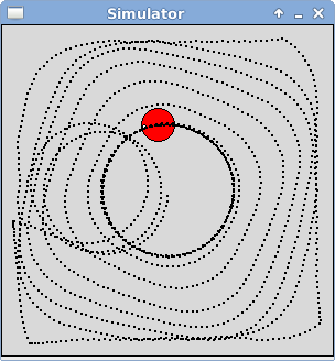

   

   0 0 0 1 1 1 1 1 1 1 1 1 1 1 0
   0 1 1 1 1 1 1 1 1 1 1 1 1 1 0
   0 1 1 1 1 1 1 1 1 1 1 1 1 1 1
   1 1 1 1 1 1 1 1 1 1 1 1 1 1 1
   1 1 1 1 1 1 1 1 1 1 1 1 1 1 1
   1 1 1 1 1 1 1 0 0 1 1 1 1 1 1
   1 1 1 1 1 0 1 1 0 0 1 1 1 1 1
   1 1 1 1 1 0 1 1 0 0 1 1 1 1 1
   1 1 1 1 1 0 1 1 0 0 1 1 1 1 1
   1 1 1 1 1 1 1 1 0 1 1 1 1 1 1
   1 1 1 1 1 1 1 1 1 1 1 1 1 1 1
   1 1 1 1 1 1 1 1 1 1 1 1 1 1 1
   1 1 1 1 1 1 1 1 1 1 1 1 1 1 1
   1 1 1 1 1 1 1 1 1 1 1 1 1 1 1
   0 1 1 1 1 1 1 1 1 1 1 1 1 1 0
   

   To implement this you'll need to modify the Agent class:
   • Modify the constructor
     Add class variables called self.gridSize and self.grid. If the grid size is 10 and the world size is 300 by 300, then each grid location is representing a 30x30 patch of the world. If the grid size is 15 and the world size remains the same, then each grid location is representing a 20x20 patch of the world. The grid is a two-dimensional list (based on the grid size) representing where the agent has visited. Each grid location should be initialized to 0.
   • Create a showGrid method
     Print the grid in an easy to view format as shown above. Test that your constructor is working properly for different grid sizes using this method.
   • Create a percentVisited method
     Sum up the 1's in the grid and return the percentage of the entire grid that has been visited.
   • Create an updateGrid method
     Using the agent's current x, y location, the grid size, and the world's width and height, update the appropriate row and column of the grid with a 1.
   • Modify the translate method
     After checking whether the agent is stalled, call the updateGrid method.
   Test that the coverage feature is working using a variety of grid sizes, world sizes, and brains. Use git to add, commit, and push your changes.

Open the file evolveVacuum.py. This program performs one evolutionary run of NEAT for the coverage task (what a robot vacuum would need to solve). Notice at the top of this file that it imports your simulator as well as a number of different classes from the neat library, including population, chromosome, genome, and nn (for neural network).

The first thing that happens in the main program of evolveVacuum.py is loading a configuration file called vacuum_config. Open this configuration file and consider all of the different parameters that need to be set for a NEAT run. In the phenotype section you set features of the neural networks that can be evolved such as the number of inputs and outputs, whether the network is feedforward, as well as the activation function. In the genetic section you set the features of the evolution such as the size of the population and the maximum possible fitness value, as well as the probabilities for certain types of mutations. In the last two sections you set features that determine how compatibility is calculated and species are formed.

Go back to the file evolveVacuum.py. The line population.Population.evaluate = ... is where you provide the name of a function that will compute the fitness values of every member of the population. I have provided a function called coverageFitness to do this for the vacuuming task.

In the coverageFitness function, notice that for each individual in the population, we open a simulator world, put an agent at the center of the world, create a neat-based brain for it, allow the agent to move for a fixed number of steps, and then use the percent of the world visited as its fitness value. Notice that this does NOT make the agent visible, allowing evolution to run much faster.

Back in the main program, the line pop.epoch(...) is what starts a NEAT evolution. The first parameter specifies the maximum number of generations to run, which is currently set to 10.

Take a look at the neatBrain defined at the end of the evolveVacuum file. Notice that the constructor creates the neural network described by the given chromosome. The select action method passes the sensor data in as input, and uses the network's output to control the agent's movement.

Now that you have an overview of how to set up a NEAT evolution. Go to a terminal window and start the NEAT evolution process:

$ python evolveVacuum.py

This will produce a number of messages detailing the progress of the evolutionary run. For each generation you will see average fitness, best fitness, number of species, and information about each species. If evolution finds the a network that achieves the maximum fitness value it terminates, otherwise it completes all of the specified generations.

Executing evolveVacuum.py will generate two files with a .svg extension. These can be viewed using xv:

1. A graph of the average and best fitness over time: avg_fitness.svg
2. A depiction of how the speciation changed over time: speciation.svg

View these graphs and note in the first graph at which generations the best fitness improved.

Executing evolveVacuum.py will generate files storing the chromosome of the best network from every generation of evolution. We need a way to test out these networks to see what NEAT has created. Open the file evaluateVacuum.py. This program begins by taking in a command-line argument specifying a saved chromosome file, then what follows is similar to evolveVacuum.py. It loads the configuration file, and then sets up the simulator, but this time with a visible agent with the trail turned on so that we can see how well the agent evolved to cover the world.

Using this program we can test out any one of the saved best networks by doing the following and replacing n with the appropriate generation number:

$ python evaluateVacuum.py best_chromo_n

Try this starting with generation 0 and then looking at other generations where the best fitness improved. The evaluateVacuum.py program will print a description of the nodes and connections of the given chromosome file, and show you the agent using the neural network described by this chromosome file running in a visible graphics window.

Executing this program also generates a file to help you visualize the network structure. To see a visualization of the network from generation n do:

$ xv phenotype_best_chromo_n.svg

Try running the entire evolution process again. How do the results differ between runs?

When using NEAT, many parameter settings must be specified and it isn't always clear how best to make these choices. In the final section of this lab you will conduct a series of experiments and write up your results. Each of the choices made in the code above could affect the types of behavior that will be evolved. Below are just some of the parameter settings that you could explore. Focus on just one or two modifications.

• What inputs should be provided?
  In the original code only two were given: the stall and a normalized distance to the wall. Would the evolved behavior change if we also provided the current coverage as an additional input? Are there other inputs that you could add to your simulator that would be helpful?
• How should fitness be measured?
  In the original code we used a grid size of 15 and the percent visited as the fitness. How would things change if we made the grid size bigger or smaller? Is there another method of evaluating coverage rather than percent visited?
• How should the NEAT parameters be set?
  Should the probability of adding nodes and connections be changed? Should more or less speciation be encouraged? Should we use bigger populations and run for more generations?

Write a short paper describing your experiment. You should conduct at least 10 experiments using the original framework I provide and calculate the average fitness achieved and save screen shots of the types of behavior discovered. Then conduct the same number of experiments using your revised framework, again calculating the average fitness and types of behavior found. Compare and contrast the original results to the outcome of your changes. Be sure to include images of the screen shots in your paper.

Hand in a printout of your paper at the next lab meeting.

When you are completely done, be sure that you have pushed all of your changes to the repo. Use the git status command to verify this. If there are uncommitted changes, be sure to do another add, commit, and push cycle.