This week, we will again be using the Pac-Man interface developed by John DeNero and Dan Klein at UC Berkeley.
You are encouraged to work with a partner on this lab. Please read the following instructions carefully.
If you want to work alone do:
setup63-Lisa labs/08 noneIf you want to work with a partner, then one of you needs to run the following command while the other one waits until it finishes:
setup63-Lisa labs/08 partnerUsernameOnce the script finishes, the other partner should run it on their account.
cd ~/cs63/labs/08
cp -r /home/bryce/public/cs63/labs/08/* .
git add *
git commit -m "lab8 start"
git push
cd ~/cs63/labs/08
git pull
In this lab, you will explore variations on two algorithms you have encountered before: Q-learning and Monte Carlo tree search.
Your first task is to implement UCB selection as an exploration policy for Q-learning. You will then re-implement MCTS in the context of reinforcement learning, both as an offline and online MDP solver.
Many of the files you have copied to your directory are the same as last week, but some have been modified to play nicely with MCTS. All of the code you write will go in UCBAgents.py.
Last week, you implemented Q-learning with an epsilon-greedy exploration policy. This policy has some shortcomings that we will attempt to improve upon:
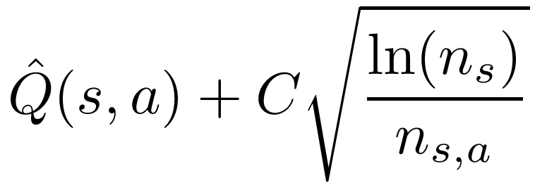
We have already encountered an exploration policy that can alleviate these issues. UCB computes a weight for each option according to its estimated value and the number of times it has been explored. In the following formula for the UCB weight, n_s is the number of times the state has been seen, and n_s,a is the number of times the action has been taken in that state.
Computing UCB weights requires us to keep track not only of the estimated Q-values, but also the number of times each (state, action) pair has been seen. Analagous to Q-values, we don't need to keep track of visits to each state, because we can compute as the sum of the state's action's visits.
Important to remember: In order to use the above formula to compute probabilities, the weights must be non-negative. You can adjust for this by calculating all of the weights and then finding the minimum weight. If it is less than 0, then add the abs(min weight) to every weight. Once all of the weights are non-negative you can normalize them.
Also note: Another case you need to consider is when the weights are all 0. This can occur when the Q values for that state are all 0 and the particular state, action pair has only been visited one time, making the log calculation also 0. In this case, simply choose one of the actions randomly.
UCB weight can be used to select actions during exploration in two different ways. In lab 4, we selected an option randomly with probability proportional to the UCB weights. On the other hand, Monday's reading suggests deterministically selecting the action with the highest UCB weight. You should try out both of these methods to see which works best.
In UCBAgents.py, you need to finish implementing the class UCB_QLearningAgent. Luckily, you've already done a lot of the work in lab 7. The following methods for the UCB_QLearningAgent class should work if copied from your lab 7 QLearningAgent class.
The following methods should be able to reuse most of the code from QLearningAgent, but will also need to keep track of the number of visits. The getVisits function is analogous to getQValue.
The getAction method has been implemented for you, and calls the new method UCB_choice which you will need to implement. UCB_choice computes UCB weights for each legal action from the current state and then returns either the max-weight action, or a random action drawn with probability proportional to weights. The variable self.randomize selects between these two versions. You should test both versions to see which is more effective in each environment.
You can run your UCB_QLearningAgent on both the gridworld and PacMan domains with the following commands.
NOTE: If running these tests remotely, you may want to add the -q flag for quiet mode, which will skip the graphics simulation.
python gridworld.py -a q -k 100 -g BookGrid -u UCB_QLearningAgent

python pacman.py -p PacmanUCBAgent -x 2000 -n 2010 -l smallGrid
Remember from last week that both domains have a number of available layouts.
Next, you'll be taking things a step further and using MCTS to solve the MDP. Interestingly, MDP solving (not complete-information game playing) was the original purpose for which the UCT algorithm was proposed.
In lab 4, we used MCTS to make online decisions, where the agent ran MCTS at every node where it needed to make a decision. For this lab, you will first implement MCTS for offline learning, where the agent will explore and learn values using MCTS, but will then freeze its value estimates and use a greedy policy for testing.
The OfflineMCTSAgent class you will be implementing inherits from UCB_QLearningAgent, so that the following functions can be reused:
In addition, depending on your implementation, it may be possible to reuse the following functions. Their overriding definitions are commented out in OfflineMCTSAgent, but if you need to define them, you may.
In addition, the update function for OfflineMCTSAgent has been implemented for you. Your task is to implement selection, expansion, and backpropagation for Monte Carlo tree search. Note that because we do not have separation between the agent's environment and a simulator of that environment, we are omitting the simulation step. However, the result of repeated expansion operations on new states has an effect similar to simulation, albeit with higher memory overhead.
The selection function plays a similar role to the UCB_choice function in UCB_QLearningAgent, in that it is called by getAction during the exploration phase and it selects an action according to UCB weights computed from stored Q-values and visit counts. As before, the variable self.randomize determines whether to return the the highest weight action or a weighted random action. This function is also responsible for updating the visit count for each action that it selects.
However, selection has the additional task of storing each (state, action) pair it encounters in the self.history list. In addition, to emphasize the phases of the MCTS algorithm, expansion has been broken out into a separate function. You are encouraged, but not required, to identify common functionality and design your code so that it can be inherited.
When selection is called on a state where not all actions have been tried, it cannot compute UCB weights, and instead calls expansion. Expansion selects an action uniformly at random among those that have not yet been visited. It must ensure that the expanded state and action are added to both the Q-values and visits tables.
In Monte Carlo tree search, we don't update the value esimates at every timestep, so the update function that has been provided for you simply appends the reward observations to a list for later use. The backpropagation function gets called when a terminal state is encountered. At this point the value estimate of every (state, action) pair encountered in the rollout gets updated. Unlike Q-learning, there is no learning rate parameter, so the value estimate is simply the average future reward across all instances where a (state, action) pair was encountered.
To update the estimated values of the state, action pairs seen in one episode, you first need to calculate the discounted reward received over the rest of the rollout after a particular state, action was visited. For a state and action encountered at time T, the discounted future reward is
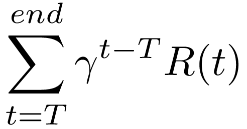
where gamma is the discount rate, and R(t) is the reward at time t. This sum is easy to compute by iterating over the rewards in reverse order. Here is a simple example that demonstrates how the discounted reward is calculated.
To correctly update the Q-value, we need to know the number of times each state, action pair was encountered in the current rollout. Call this value the new ns,a. We also need to know the number of times the pair was seen across all previous rollouts; call this the old ns,a. The new count can be determined by the number of times (s,a) appears in the history list. The old count is the difference between the total nubmer of visits to (s,a) and the new count. Updating the average value then works as follows:
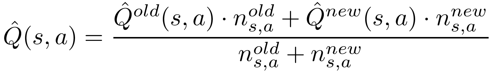
Where the new Q is the average discounted future reward across all occurrences of (s,a) in the current rollout, and the old Q is stored in Q_table.
After all value estimates have been updated, backpropagation should reset self.history and self.rewards to empty lists for the start of the next rollout
NOTE: If running these tests remotely, you may want to add the -q flag for quiet mode, which will skip the graphics simulation.
python gridworld.py -a q -k 100 -g BookGrid -u OfflineMCTSAgent

python pacman.py -p PacmanMCTSAgent -x 2000 -n 2010 -l smallGrid
In the Pac-Man world, the results can be quite variable. In my tests (using a self.discount = 0.9), the worst performance has been 4 wins in 10 trials, the best has been 9 of 10, with an average of about 7 in 10. The default setting for the discount in the Pac-Man world is 1.0, which you should definitely override.
The following starting point files in /home/bryce/public/cs63/labs/08/ have been updated:
To get started on this task, you should copy over the new gridworld.py file, replacing the old one. You should then open UCBAgents.py in an editor and copy over the starting point code for the OnlineMCTSAgent class (lines 206-307).
In contrast to the offline version, which starts all rollouts from the start state of the MDP, an online Monte Carlo tree search agent runs simulated rollouts from every node where it needs to make a decision. This requires access to a simulator that can predict the outcomes of those actions. The new version of gridworld.py implements such a simulator, which provides two methods:
The selection function has been implemented to call the version you implemented in OfflineMCTSAgent and then get the action's result from the simulator, saving the reward, and returning the next state. The expansion function has also been provided, relying again on a call to your OfflineMCTSAgent implementation. Your task is to implement the two remaining components of MCTS and also a function that puts the pieces together:
The simulation function takes over after a new (state, action) pair has been expanded and runs the remainder of the rollout by taking uniformly random actions. At each state encountered, a uniformly random legal action is selected. The simulator is then used to generate a next state and a reward. The reward is appended to self.rewards, but the state and action are not saved in self.history. The rollout continues until either 1) a terminal state is reached, or 2) self.rewards has length equal to the self.depth_limit.
The backpropagation function should call the version you wrote for OfflineMCTSAgent, but should first update self.rewards to have the same length as self.history. The updated rewards list will have all rewards from the simulation phase compressed into the final entry. That is, self.rewards[-1] will be the reward at the expanded (state, action) pair, plus the sum of discounted rewards over the whole simulation phase.
The MCTS function puts all of the pieces together. This is the function called by getAction, but it does not need to return an action. Instead, it updates the Q_table, after which getAction calls computeActionFromQValues to pick the best action according to the simulation estimates. MCTS runs a number of rollouts determined by the self.rollouts field. Each rollout consists of repeated calls to selection, followed by one call to simulation and one call to backpropagation (expansion is called automatically). The simulation phase continues until a new (state, action) pair is expanded (indicated by the self.selecting flag being set to False). The self.depth_limit field gives the maximum number of actions that should be taken over the course of a rollout (including selection, expansion, and simulation phases). A rollout ends when either a terminal state or the depth limit is reached, regardless of which phase the algorithm is in.
You can test your online MCTS agent on any of the gridworld layouts with commands like the following. Unfortunately, we don't have a simulator class for the agent to use to run online MCTS in the PacMan domain.
gridworld.py -a q -k 50 -g NineByFive -u OnlineMCTSAgent -d 0.9
cd ~/cs63/labs/08
git add UCBAgents.py
git commit -m "final version"
git push