Lab 5: Neural networks

Lab 5: Neural networks
Due March 15 at the start of lab

On the left, an image of a person wearing sunglasses. On the right, an image representing the weights of a hidden unit in a neural network trained to classify such images.

Starting point code

This lab may be done alone or with a partner of your choice. Go through the following steps to setup your directory for this lab.

First you need to run setup63 to create a git repository for the lab. If you want to work alone do:
```
setup63-Lisa labs/05 none
```
If you want to work with a partner, then one of you needs to run the following while the other one waits until it finishes.
```
setup63-Lisa labs/05 partnerUsername
```
Once the script finishes, the other partner should run it on their account.
For the next step only one partner should copy over the starting point code.
```
cd ~/cs63/labs/05
cp -r ~meeden/public/cs63/labs/05/* ./
```
This will copy over the starting point files for this lab.
Whether you are working alone or with a partner, you should now add all of the files to your git repo, commit, and push them as shown below.
```
git add *
git commit -m "lab5 start"
git push
```
If you are working with a partner, your partner can now pull the changes in.
```
cd ~/cs63/labs/05
git pull
```

Introduction

In this lab you will use neural networks on a number of classification tasks. First you will explore using neural networks to solve some of the simpler problems we discussed in class such as the logic problems AND, OR, and XOR. Next you will look at an auto-encoder problem where the network develops a binary-like representation in its hidden layer. Then you will experiment with a handwritten digit recognizer. Finally you will focus on classifying images of faces.

You will be writing up your answers to this lab as a LaTeX document. The repo contains a starting point document for you in the file lab5.tex. In order to convert the LaTeX document into a pdf and view it do:

pdflatex lab5.tex
evince lab5.pdf

You should track the LaTeX document in git. However, you should NOT track the resulting pdf file that you create. You will also be creating some short programs to set up and run your own classification task.

File that will be evaluated:
`lab5.tex`	Your answers to all of the lab questions go here
Files you'll use:
`and-net.py`	Creates a two-layer network to solve AND
`or-net.py`	Creates a two-layer network to solve OR
`xor-net.py`	Creates a two-layer network that is unable to solve XOR
`xor-3layer.py`	Creates a three-layer network to solve XOR
`inputs.dat`	Contains the four input patterns used for all of the logic problems
`and-targets.dat`	Contains the four target patterns for AND
`or-targets.dat`	Contains the four target patterns for OR
`xor-targets.dat`	Contains the four target patterns for XOR
`8bit-net.py`	Creates a three-layer auto-encoder network
`8bit.dat`	Contains the eight input and target patterns for the auto-encoder problem
`digit-net.py`	Creates a three-layer network to classify handwritten digits
`digit-inputs.dat`	Contains the input patterns for the digits classifier
`digit-targets.dat`	Contains the target patterns for the digits classifier
`glasses-net.py`	Creates a three-layer network to classify images of people's faces
`sunglassesfiles`	File names of the images to be used to create the glasses training set (you will create this)
`glasses-inputs.dat`	Contains the input patterns for the glasses classifier (you will create this)
`glasses-targets.dat`	Contains the target patterns for the glasses classifier (you will create this)
`processingFaces.py`	A collection of functions to convert the raw image data into a form usable by a neural network
Supporting files you can read, but should not modify:
`conx.py`	Implements neural networks
`newConx.py`	Enhances the original conx code by providing visualization

Using the neural network libraries

You should review the summary of neural network library methods before you begin.

Solving logic problems

In this section you will explore how neural networks perform on the basic logic problems AND, OR, and XOR. For these problems there are just four different input patterns (the x's), as shown in the table below:

x₁	x₂	AND(x₁, x₂)	OR(x₁, x₂)	XOR(x₁, x₂)
0	0	0	0	0
1	0	0	1	1
0	1	0	1	1
1	1	1	1	0

Open the program and-net.py in an editor. Read through the code first, then try executing it to create a simple network to solve AND:
```
python -i and-net.py
```
Note that using the -i option when invoking python will execute the given filename and then leave you in the interpreter. It has just two inputs and one output, along with a bias. Before training, test the AND network's performance and look at its weights. Then train the network and re-test its performance and check out how the weights have changed. Do the weights make sense to you? Draw a picture of the network if that helps you visualize the solution. Exit from the interpreter.
Next create a simple network to solve OR:
```
python -i or-net.py
```
It has the same structure as the previous network. Try all of the same commands as before. Make sure that the learned weights make sense to you. Exit from the interpreter.
Then create a simple network to try to solve XOR:
```
python -i xor-net.py
```
Again it has the same structure as the previous two examples, however when you train this network it will be unable to learn. You can do CTRL-C to interrupt the training. Exit from the interpreter.
Finally create a more complex network that can solve XOR:
```
python -i xor-3layer.py
```
In this case the network has three layers (input, hidden, and output) instead of just two (input, output). To see all of the weights for this network requires two commands:
- n.printWeights('input','hidden')
- n.printWeights('hidden','output')
After training this three-layer XOR network, use the above commands to inspect the final learned parameters. Edit the diagram of the network in the file lab5.tex to show all of the trained weights and biases. Then explain in the writeup how the network has solved the problem based on them.
Remember that each unit in the network computes the following (where the x's represent the incoming activations and the w's represent the incoming weights): :
```
netInput = bias + Σx_iw_i
output = f(netInput)
```
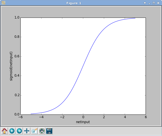
The default activation function f in this neural network library is the sigmoid: 1/(1+e^-netInput) which is plotted below. So for example if the netInput for a particular unit is 0, it would output the value 0.5. The more negative the netInput, the closer the output gets to 0. The more positive the netInput, the closer the output gets to 1.

Analyzing hidden layer representations

Look at section 4.6.4 starting at the bottom of page 106 in Tom Mitchell's Chapter 4 about hidden layer representations. We will be using bit patterns where a single bit is set to 1 and the rest are set to 0. We will focus on bit patterns of length 8 as discussed in the reading, so there are only 8 possible patterns.

Create a network that learns to take eight-bit patterns and reproduce them on the output layer after re-coding them in a three-unit hidden layer:

python -i 8bit-net.py

After training, use the showPerformance() method to inspect the hidden layer representations. In the file lab5.tex write down each of the hidden layer representations created by the network in the table provided. Then convert them into bit patterns by rounding each hidden unit activation to either 0 or 1. Discuss whether the network re-coded them using a binary-like representation.

Classifying handwritten digits

Create a network that learns to classify handwritten digits:

python -i digit-net.py

When you run this file it will open up additional windows so that you can visualize the input, hidden, and output activations as well as the hidden weights. Move the windows around so that you can see all of them. Each individual activation or weight is depicted as a grayscale box. The lighter the color the higher the value, the darker the color the lower the value.

This network takes 8x8 images as input, passes them through a 5-unit hidden layer, and classifies them in a 10-unit output layer. Each unit in the output layer is associated with one digit (0-9). For example, if the last unit is highly active, this means that the network is classifying the current image as the digit 9. In contrast, if the first unit is highly active, this indicates the network is classifying it as the digit 0.This data set contains 100 examples including images of:

10 zeros
11 ones
11 twos
11 threes
12 fours
5 fives
8 sixes
12 sevens
9 eights
11 nines

This is the first data set in the lab where we've had enough data to create both a training set and a testing set. Notice that the splitData method has been used to randomly select 60% of the data set for training. You should train for a limited number of epochs, say 25, swap the data and evaluate the network's performance on the testing set. Continue swapping and training as long as the performance on the testing set is improving.

Pick one digit to focus on and analyze it in more depth. Choose one that has a reasonable number of examples in the training set. Find every instance of that pattern in the training set and record which hidden units are active (0-4) in the table provided in the file lab5.tex. Look at the hidden layer weights in the displays. In lab5.tex describe how the network learned to recognize this digit based on the hidden layer features it has discovered. Include images of the hidden weights, if you'd like.

Classifying images

We will be using the same images of faces that were discussed in this week's reading. Look at section 4.7 from Tom Mitchell's Chapter 4 (pages 112-116).

The directory /home/meeden/public/cs63/faces_4/ contains 624 images stored in PGM format. Do NOT copy these images to your own directory. You can view one of these images using the xv command. Each file is named according to the following convention:

userid_pose_expression_eyes_scale.pgm

userid is the user id of the person in the image. This field has 20 values: ani2, at33, boland, bpm, ch4f, cheyer, choon, danieln, glickman, karyadi, kawamura, kk49, megak, mitchell, night, phoebe, saavik, steffi, sz24, and tammo.
pose is the head position of the person, and this field has 4 values: straight, left, right, and up.
expression is the facial expression of the person, and this field has 4 values: neutral, happy, sad, and angry.
eyes: is the eye state of the person, and this field has 2 values: open and sunglasses.
scale: is the scale of the image. All of the images are of type 4 which indicates a quarter-resolution image (32 x 30).

Using a neural network to learn a classification task involves the following steps: determining a task, gathering appropriate data, creating the training set of inputs and targets, creating a network with the appropriate topology and parameter settings, training the network, and finally analyzing the results. Each of these steps is explained in more detail below. After you have tried these steps on the sunglasses example, you will repeat this process on a task of your choosing.

Choose a task
The first step is deciding what classification task you would like to learn. There are a number of possibilities such as presence of sunglasses, head position, emotion, or identifying particular individuals. Some of these classification tasks will be easier to learn than others. As an example, let's focus on the relatively easy task of determining whether or not a person is wearing sunglasses.

Gather data
Next we need to select which of the images to use in our training set. As a starting point, let's focus on images where the person is looking straight ahead and has a neutral expression. We need to gather together all of the filenames that meet these criteria. We can use ls with the -C1 flag to ensure that the output from the listing is in one column. We can choose appropriate files with the wildcard *, and then use the greater than sign to save those image file names into a file in our own directory:
```
cd /home/meeden/public/cs63/faces_4
ls -C1 *straight*neutral* > ~/cs63/labs/05/sunglassesfiles
```
Using the unix command wc ~/cs63/labs/06/sunglassesfiles we can see that this file has 40 lines in it. We may want a slightly larger training set. So let's add in all the images where a person is looking straight ahead and has a happy expression. We can do this by again using ls to select these images and using two greater than signs to append these additional names to the end of the same file:
```
ls -C1 *straight*happy* >> ~/cs63/labs/05/sunglassesfiles
```
Using the wc command again we see that we now have 79 images. Once your sunglasses file is correct, use git to add, commit, and push it.
Create training set
Once we have selected a good set of images, we need to convert them into a format that is appropriate for the neural network. The PGM files have pixel values between 0 and 255; we need to normalize these values between 0 and 1. In addition, we need to create input files where each normalized image is written one per line. Some python functions have been provided in the file processingFaces.py to help you prepare these image files:
- The function getImages takes a directory name where the images are stored, a filename containing the names of image files in that directory, and a filename to put the normalized image values.
- The function getTargets takes a filename containing the names of image files, and a filename to put the target values for the task. It uses some aspect of the filename to determine an appropriate target value. In the sunglasses example, if it finds the word 'sunglasses' in the filename, then the target value should be 1. Otherwise the target value should be 0.

Execute this file by doing:

python processingFaces.py

glasses-inputs.dat

glasses-targets.dat

wc

Set up network
Once the training data has been prepared we can create the neural network, as provided in the file glasses-net.py. This creates a new class called SunglassesRecognizer that inherits from the class BackpropNetwork. It adds two additional methods classify and evaluate. At the bottom of the file, it sets up the network:
- First it creates an instance of the class. Then it creates a three-layer neural network with 960 inputs (to represent the 32 by 30 pixel values in each image), 1 hidden unit, and one output unit. For harder tasks you will need more hidden units. For tasks with more categories, you will also need an output unit for each category.
- Then it sets the learning parameters (epsilon, momentum, and tolerance).
- Next it creates windows to show the activations of all of the layers in the network, as well windows to display all of the weights from the input to the hidden layer.
- Finally, it randomly splits the data into a training set and a test set. Typically you will want to use about 75-85 percent of the data for training, and the remainder for testing.
Execute this file by doing:
```
python -i glasses-net.py
```
This will produce a number of windows. Move them around so that you can see them all.

Train network
One of the advantages of using neural networks is their generalization ability. We want to train the network using the training set, but we don't want the network to memorize the training set. We want the trained network to be able to respond appropriately to novel input. We need to be careful not to over train the network. Thus the goal is not to achieve 100 percent correctness. We will train the network for a number of epochs and then test the network on novel data to monitor how well it is generalizing. We will repeat this process until the network is no longer improving its performance on the novel data. For example, try the following commands in the python interpreter after you have set up the network:

>>> n.train(5)
Epoch #     1 | TSS Error: 15.3588 | Correct: 0.0000
Epoch #     2 | TSS Error: 15.2270 | Correct: 0.0000
Epoch #     3 | TSS Error: 15.2524 | Correct: 0.0000
Epoch #     4 | TSS Error: 15.1156 | Correct: 0.0000
Epoch #     5 | TSS Error: 14.8360 | Correct: 0.0000
Reset limit reached; ending without reaching goal
----------------------------------------------------
Final #     5 | TSS Error: 14.8360 | Correct: 0.0000
----------------------------------------------------

You can see that error is dropping, but so far the network has not learned to respond correctly to any of the training patterns. NOTE: because each network is initialized with different random weights your training results will vary. Let's check on how well the network is doing on the test patterns.

>>> n.swapData()
Swapping training and testing sets...
19 training patterns, 60 test patterns
>>> n.evaluate()
network classified image #0 (sunglasses) as ???
network classified image #1 (sunglasses) as ???
network classified image #2 (eyes) as ???
network classified image #3 (sunglasses) as ???
network classified image #4 (eyes) as ???
network classified image #5 (eyes) as ???
network classified image #6 (eyes) as ???
network classified image #7 (eyes) as ???
network classified image #8 (eyes) as ???
network classified image #9 (eyes) as ???
network classified image #10 (sunglasses) as ???
network classified image #11 (sunglasses) as ???
network classified image #12 (eyes) as ???
network classified image #13 (eyes) as ???
network classified image #14 (eyes) as ???
network classified image #15 (eyes) as ???
network classified image #16 (eyes) as ???
network classified image #17 (sunglasses) as ???
network classified image #18 (eyes) as ???
19 patterns: 0 correct (0.0%), 19 wrong (100.0%)

As expected, it is not responding correctly to these either. Let's swap the data back, continue training, and then re-test.

>>> n.swapData()
Swapping training and testing sets...
60 training patterns, 19 test patterns
>>> n.train(5)
Epoch #     1 | TSS Error: 14.2245 | Correct: 0.0000
Epoch #     2 | TSS Error: 12.9923 | Correct: 0.0000
Epoch #     3 | TSS Error: 10.3263 | Correct: 0.0000
Epoch #     4 | TSS Error: 7.8044 | Correct: 0.0833
Epoch #     5 | TSS Error: 5.8430 | Correct: 0.3500
Reset limit reached; ending without reaching goal
----------------------------------------------------
Final #     5 | TSS Error: 5.8430 | Correct: 0.3500
----------------------------------------------------
>>> n.swapData()
Swapping training and testing sets...
19 training patterns, 60 test patterns
>>> n.evaluate()
network classified image #2 (eyes) as ???
network classified image #4 (eyes) as ???
network classified image #5 (eyes) as ???
network classified image #6 (eyes) as ???
network classified image #7 (eyes) as ???
network classified image #8 (eyes) as ???
network classified image #9 (eyes) as ???
network classified image #10 (sunglasses) as ???
network classified image #12 (eyes) as ???
network classified image #13 (eyes) as ???
network classified image #14 (eyes) as ???
network classified image #15 (eyes) as ???
network classified image #16 (eyes) as ???
network classified image #18 (eyes) as ???
19 patterns: 5 correct (26.3%), 14 wrong (73.7%)

Clearly the performance of the network is improving. After several more iterations of this process of swapping the data and additional training, the network will start performing well on both the training set and the testing set and learning can be stopped. Remember the goal is to achieve good performance on the training set while still being able to respond appropriately to the novel data in the testing set.

Analyze results
Once the training process is complete, we can look more closely at the activations and weights to try to understand how the network has solved the task. In the python interpreter do n.showPerformance() and observe for which images each unit is active. How are the hidden units coding for the different categories of images? For the sunglasses task there is only one hidden unit, so this is pretty straight forward. Next look at the hidden weights. What parts of the image are the hidden units focusing on? Why are these locations of the image important for the given task?

After you have successfully completed the sunglasses example, repeat this process (Steps 1-6 above) on a task of your choice using some subset of the faces image data. In the file lab5.tex explain in detail what you did in each step.

Creating a successful classifier often requires an iterative process. You may find that you need more hidden units. You may find that you need more training examples. Some problems you'd like to try (such as recognizing the emotions in the images) may be too difficult to solve with these down-sized images.

Once you have successfully created a new classifier, take screen shots of your resulting hidden weights and save them in files called hidden1.png, hidden2.png, and so on.

One method of getting screen shots is to right click the mouse on the camera icon at the bottom of your screen. Select properties and then select "Active Window" under "Region to capture". You will only need to do this step once. From now on, it will always grab the active window. Then go to one of the conx weight windows and left click the mouse to make it the active window. Finally left click on the camera to get the screen shot. Include these hidden files as figures in your lab writeup.

Submitting your code

To submit your code, you need to use git to add, commit, and push the files that you modified. Print out the pdf version of the lab5.tex file and hand it in at the start of lab the Tuesday after spring break (March 15).