LAB DUE DATE:Thursday, October 1st, 11.59PM
1. Membership Inference and Model Extraction
This lab shifts the attacker’s goal from causing incorrect predictions (Labs 2 and 3) to learning private information or copying a model’s behavior through its prediction interface.
-
Membership Inference Attack (MIA): The attacker submits a candidate record and examines the model’s output to infer whether that record was used to train the model. The goal is to discover the record’s participation in training, not, to recover an unknown training record.
-
Model extraction: The attacker submits many inputs, collects the model’s predictions, and uses those input–prediction pairs to train a substitute model that behaves similarly to the target. Note that model extraction is about copying functionality; it does not automatically reveal a person’s training record.
In both attacks, the attacker uses ordinary prediction queries. The attacker does not need to modify the target’s training data or access its internal parameters.
-
Attack vector: The model’s prediction interface. The attacker submits inputs and uses the returned probabilities or labels to infer membership or train a substitute.
-
Trust assumption: Providing predictions preserves the privacy of training-set participation and protects the model’s predictive capability from copying.
-
Security question: Does that assumption hold? What can an attacker learn or reproduce using only the permitted outputs?
2. Objectivies
By the end of this lab, you should be able to:
-
implement a membership score and a decision threshold calibrated with shadow data;
-
distinguish a target model, shadow model, membership decision rule, and extracted substitute;
-
distinguish task accuracy, membership inference performance, and extraction fidelity;
-
interpret false positives and false negatives via examples;
-
understand how output restriction works, and and what an adaptive attacker can still do; and
-
connect this lab to security principles: understanding assets, trust boundaries, and principles of least privilege, and defense in depth.
3. Attack Model
| Security Goals | Lab 3: SVM poisoning, BadNets, and Poison Frogs | Lab 4: membership inference and model extraction |
|---|---|---|
Attack Objective |
SVM poisoning: degrade classification performance. BadNets: make inputs carrying a trigger receive the attacker’s chosen label. Poison Frogs: make a particular target input receive an incorrect label using clean-label poisoned training examples. |
Membership inference: determine whether a candidate record trained the target. Model extraction: train a substitute that reproduces the target’s predictions. |
Security Triad Affected (CIA) |
SVM poisoning: integrity of the learned classifier; broad degradation can threaten availability. BadNets and Poison Frogs: integrity of selected predictions. |
Membership inference: confidentiality of training-set participation. Model extraction: confidentiality of a protected model capability, by copying its behavior. |
Trust Assumption Being Challenged |
Training examples are safe to learn from. Correct labels alone do not guarantee this: clean-label poisons can still manipulate learning. |
Providing predictions preserves the privacy of training membership and does not enable users to copy the model’s behavior. |
Attacker’s Insight |
SVM poisoning: carefully chosen training points can shift the decision boundary. BadNets: a model can learn an association between a trigger and a chosen label. Poison Frogs: a poison can resemble one class to a person while resembling the target in the model’s feature representation. |
Membership inference: the model’s confidence may differ between training members and nonmembers. Model extraction: the target’s predictions can serve as training labels for a substitute. |
Attack Entry Point |
Before or during training, through poisoned training examples. |
After training, through the target’s prediction interface. |
Attacker-Controlled Data |
SVM poisoning: injected training points, subject to the attack’s constraints. BadNets: trigger-bearing training examples and their assigned labels. Poison Frogs: the pixels of selected poison examples, while retaining their correct labels. |
Membership inference: candidate inputs submitted to the target. Model extraction: query inputs and the substitute’s training process. The target supplies the query labels. |
Changes to the Underlying Target Model |
Yes: each attack changes what the target learns from its training data. |
No: the target remains fixed. Extraction trains a separate substitute. |
Evidence of Attack Success |
SVM poisoning: increased error on clean test data. BadNets: trigger-bearing inputs receive the chosen label while clean accuracy may remain high. Poison Frogs: the selected target is misclassified while overall accuracy may remain high. |
Membership inference: membership guesses outperform chance on a balanced evaluation set. Model extraction: the substitute agrees with the target on held-out inputs, including cases where the target is wrong. |
4. Part 0: Setup and threat model
4.1. Datasets and model choice
The default is MNIST, using your existing mnist.npz. You must also run your results with:
-
Fashion-MNIST: 28-by-28 grayscale clothing images. Use
DATASET = "fashion_mnist"in the following mannerDATASET = "fashion_mnist" DATA_FILE = Path("data") / f"{DATASET}.npz" (x_train, y_train), (x_test, y_test) = fashion_mnist.load_data() -
Digits: scikit-learn’s built-in 8-by-8 handwritten digits, selected with
DATASET = "digits". It needs no dataset download and uses smaller sample counts.
The notebook uses small scikit-learn multilayer perceptrons. You already used scikit-learn in Lab 3; these attacks require predictions rather than TensorFlow input gradients. Inputs are flattened and scaled to [0,1]. Do not reuse prior labs normalized checkpoint inputs here.
We train fresh target and shadow models because membership inference requires reliable knowledge of which records were used for training.
4.2. Attacker assumptions in this lab
The target model is the classifier whose training information or behavior the attacker wants to learn. It is already trained when either attack (MIA or Model Extraction) begins. Both attackers submit images through the model’s or target’s prediction interface; neither attack changes the target’s behavior.
The table below states what information each attacker has in our lab environment. These are the assumptions for these experiments, not general requirements across MIA or mdoel extraction attacks. A query corresponds to submitting one image and receiving the target’s prediction for it.
| Capability | Membership inference | Model extraction |
|---|---|---|
Question the attacker asks |
“Did this particular image help train the target?” |
“Can I build my own model that gives the same answers as the target?” |
Information available |
Candidate images and their correct classes. Separate labeled images for training an attacker-owned practice model. Knowledge of the target’s model family and training paradigm. |
Images from the supplied query pool. The attacker knows the input format but does not use the images' correct classes. |
Observable target output |
A probability for every class. Similar to the paper, we will also we test the restriction that returns only the predicted class. |
Only the predicted class, such as “7” or “shirt.” |
Information unavailable to the attack |
The target’s internal parameters or gradients and the private training data. |
The target’s internal parameters and training data; the query images' correct classes; and final evaluation images for training. |
What an attacker can control |
Submit the candidates for prediction; train the practice/shadow model; choose a membership decision rule using that practice/shadow model’s results. |
Choose images within the query pool and budget; train a separate substitute using the target’s answers. |
Target-query budget |
One probability output per candidate: 1,200 candidates for MNIST/Fashion-MNIST or 400 for digits. Our class-only comparison is derived from the same outputs. |
Compare 100, 500, and 2,000 labeled images for MNIST/Fashion-MNIST, or 50, 200, and 600 for digits. We will queries the largest budget once and reuse prefixes for smaller experiments. |
| Submitting a batch of 100 images counts as 100 image queries, not one. Queries used by the evaluator to measure final performance are recorded separately from the attacker’s model extraction budget. |
4.3. Membership Inference Attack
Let’s understand the attack starting with the MNIST data. Assume the attacker has an image of a handwritten 7. The attacker knows what the image depicts, but does not know whether this particular image was used to train the target.
For this task, we will use two different labels:
-
A task label: that describes the image’s correct class: for example, digit
7or, in Fashion-MNIST, ankle boot. -
A membership label: that describes whether this particular image was used to train the model: member if it was in the training dataset and nonmember if not.
-
A target membership label answers this question specifically for a particular target model.
Back to our example: Classifying an MNIST image as the digit 7 does not tell the attacker whether it was used in training or not. Instead, the attacker builds a shadow model, trained on seperate but similar data to the target model and the attacker uses this model, along with the target model’s output to classify whether a particular image (in this case the digit 7) was used in training or not. The attacker’s classification is a prediction of whether the digit was used in training.
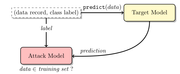
How to read this figure: The candidate image goes to the yellow Target Model, which returns probabilities for the task classes. The candidate’s correct class label and the returned probabilities go to the pink Attack Model. Its answer is “member” or “nonmember,” rather than a digit or clothing class. This diagram shows the attack process; it does not guarantee that the attacker’s guesses are correct.
4.3.1. This lab’s membership score and cutoff
This lab uses a simple rule instead of the paper’s learned attack classifier:
-
Submit the candidate image to the target.
-
Read the probability assigned to the image’s correct class. This number is the image’s membership score in our lab.
-
Compare that score with a threshold: a chosen numerical cutoff. Guess “member” when the score is at least the cutoff, and “nonmember” otherwise.
For example, suppose the target assigns probability 0.92 to class 7 for an image that really depicts a 7. Its score is 0.92. If the chosen cutoff is 0.90, the attacker guesses “member.” A score of 0.75 would produce a “nonmember” guess under the same rule.
These numbers are illustrative. A score of 0.92 does not mean a 92% probability of membership. It is the target’s probability for the correct image class. We use it as a possible clue because training images may receive higher confidence. An unfamiliar but easy classification image may also receive a high score — note that the classifier can make mistakes!
4.3.2. The shadow model: a practice target with known training membership
A shadow model is a separate classifier trained by the attacker to serve as a practice target. In this lab, it has the same model family and training recipe as the target, but learns from different images from the same dataset distribution. It predicts digit or clothing classes, just as the target does.
The attacker knows which images it used to train its own shadow model. It can therefore study two groups with known answers:
-
Shadow members: images used to train the shadow model.
-
Shadow nonmembers: images held out of shadow training.
The attacker obtains scores from the shadow for both groups and tries possible cutoffs. In this lab, it chooses the cutoff with the highest average of the member-detection rate and the nonmember-rejection rate. This average is balanced accuracy. Choosing the cutoff using these known shadow examples is called calibration.
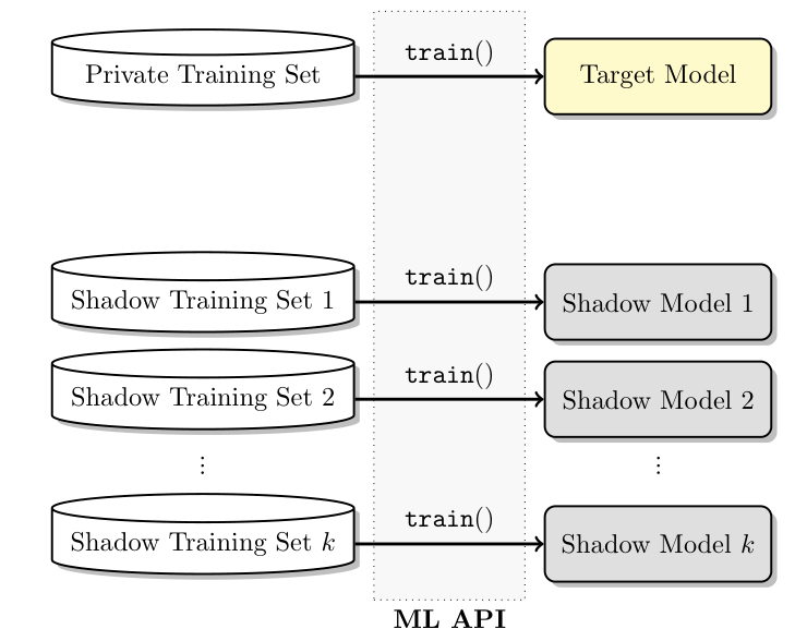
How to read the figure: The private dataset at the top trains the target. The datasets below train attacker-owned shadows. The attacker knows the shadows' training membership, even though it does not know the target’s. The paper uses multiple shadows and learns attack classifiers for individual task classes. Our lab simplifies this to one shadow model and one cutoff shared across classes. The shadow model itself is not the membership decision rule: it supplies the practice predictions used to choose that rule.
After choosing a threshold or cutoff, the attacker applies the same cutoff to the target’s scores. For example, a cutoff of 0.90 chosen on the shadow remains 0.90 when attacking the target. This is referred to as freezing the threshold. Whether a rule chosen on the shadow also works on the target is a question that the lab aims to answer.
4.4. Model Extraction
Compared to the MIA attack, a model extraction attacker has a different but related goal: the attacker’s goal is to build a substitute model, a separate classifier trained to imitate the target. It does not need to determine which images trained the target.
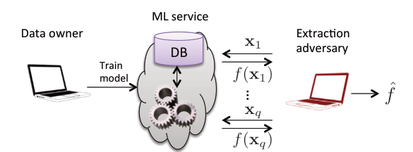
How to read the figure: The owner trains a target model behind a service interface. On the right, the extraction adversary submits inputs labeled \(x_1\) through \(x_q\). Here, \(q\) is the number of queries. The service returns predictions \(f(x_1)\) through \(f(x_q)\), where \(f\) denotes the target. The attacker uses those answers to produce its own model, \(\hat f\), which aims to behave like \(f\), the target model.
Our lab implements the attack as follows:
-
Select images from the supplied query pool, up to the allowed budget.
-
Ask the target for its predicted class for each selected image.
-
Train the substitute on those image–target-prediction pairs. Do not use the images' correct task labels.
-
Evaluate whether the substitute and target give the same predictions on separate final evaluation images.
In our MNIST dataset example, if an image actually shows the digit 7 but the target predicts 1, the extraction training pair uses 1. The attacker is learning the target’s behavior, including its possible mistakes. The percentage of evaluation images on which the two models agree is called fidelity.
The paper studies several extraction methods, including attacks that exploit confidence outputs. In this lab, we train our substitute model using the target’s answers as training labels. The goal is for the substitute model to give the same answers as the target on new images. We do not try to recover the target’s exact internal weights. In fact, the two models can give similar answers while having different internal weights.
Differences in the attacks: The two attacker-owned models have different purposes: the shadow helps choose a membership rule; the substitute is the product of extraction, trained to imitate the target’s answers.
4.5. This lab’s implementation
The notebook runs the entire experiment locally, and therefore contains information a real attacker would not have. We distinguish two roles for the attacker and the evaluator:
-
The attacker uses only the information listed in section 4.2 to choose its rule or train its substitute.
-
The evaluator checks whether the attack worked. It knows the candidates' true target membership and uses separate audit images for final model evaluation. Audit images are held-out evaluation examples, not substitute-training data.
For membership inference, the evaluator compares the attacker’s member/nonmember guesses with the target membership answer key after the cutoff has been chosen on shadow data. We do not use the target membership’s answer key to choose or revise the cutoff. Doing so would give the attacker the very information it is supposed to discover!
For extraction, the evaluator uses audit images to measure agreement and their correct task labels to measure classification accuracy. As in MIA, we do not use these images to select the substitute model. Doing so would make them part of model development rather than an independent final evaluation.
4.6. Rules for a valid attack experiment
The notebook contains the target, attacker, and evaluation code. You can therefore see information that the attacker would not have, in a real-world attack. Ensure that the following invariants are maintained, to provide you with valid results:
Rules for both attacks:
-
Do not inspect or use the target’s internal weights or gradients.
-
Do not inspect the target’s training-set list to construct the attack. A membership candidate may happen to be a training member, but the attacker must infer that fact from permitted information.
-
Do not change the target model or its training data.
Membership inference
-
You may use candidate images, their correct task labels, and the target’s returned probabilities.
-
Choose the membership cutoff using only known members and nonmembers of the shadow model.
-
Keep that cutoff unchanged when evaluating membership guesses on the target. Do not use the target’s true membership labels or its attack-evaluation results to choose or revise the cutoff.
-
In the later class-only experiment, make membership guesses using the returned class and the candidate’s correct task label, without using the target’s probabilities.
Model extraction
-
Submit only images from the supplied
query_xpool. -
Obtain target labels through
api.query(…). Do not call the target directly or inspectapi._model. -
Stay within the assigned image-query budget. Each submitted image counts as one query, including repeated images.
-
Train each substitute using only its permitted queried images and the labels returned by the target. Do not look up their correct labels in
y. -
A smaller-budget substitute must not use labels collected for a larger-budget experiment.
-
Do not use audit images, audit labels, or audit results to train, tune, or select the substitute. They are reserved for final evaluation.
Enforcing a query limit
Under “Part 4: Model extraction under a query budget,” the notebook defines a class named LabelAPI. Its query method returns predicted classes, counts submitted images, and raises an error if a request would exceed the budget.
This class enforces the extraction query limit when you use api.query(…). It does not check that images came from the permitted pool or prevent access to other notebook variables. The remaining rules above must be followed in your implementation.
Evaluator’s access rules
The provided evaluation code may use true target membership to check membership guesses, audit images, and labels to measure model performance. This information is used solely to assess the completed attacks, not to construct the attacks.
4.7. Dataset roles
The notebook divides image data into six disjoint groups. Both attacks use the same target model.
| Group | MNIST/Fashion | Digits | Use |
|---|---|---|---|
Target training |
600 |
200 |
Train the target used by both attacks. These images are also the known members when evaluating membership inference. |
Target nonmembers |
600 |
200 |
Measure target accuracy on unseen images and evaluate membership guesses on known nonmembers. |
Shadow training |
600 |
200 |
Train the membership attacker’s shadow model. |
Shadow holdout |
600 |
200 |
Provide images the shadow did not train on. Together with shadow training images, choose the membership cutoff. |
Query pool |
2,000 |
600 |
Obtain target predictions to use as labels for training extraction substitutes. |
Audit |
1,000 |
300 |
Measure final target/substitute accuracy and their agreement. Never used for training. |
Before assigning data to each partition, the notebook removes repeated copies of identical images. Our objective is to keep the class proportions approximately balanced within each group. The lab notebook then saves a manifest file mapping images to their groups.
|
Keep the seed, image groups, and model settings unchanged when comparing attacks or defenses, except for the setting you are deliberately testing. |
5. Evaluation: Fidelity, membership precision, and membership recall
To evaluate the success of our attacks we wil use three seperate metrics — Fidelity evaluates model extraction. Membership precision and recall evaluate membership inference attacks.
5.1. Fidelity: how often do the two models agree?
Suppose the substitute and target predict the same class on 90 of 100 held-out images:
Those 90 agreements could include:
-
80 images where both models give the correct answer.
-
10 images where both models give the same incorrect answer.
For example, if an image shows a 7 and both models predict 1, it belongs to the second group. It counts toward fidelity because the substitute reproduced the target’s answer. On the remaining 10 images, the models disagree. Fidelity does not tell us which model is correct on those images.
What 90% fidelity tells us: the substitute matched the target on 90% of the evaluation images.
What it does not tell us: that either model achieved 90% classification accuracy. Accuracy requires comparing predictions with the images' correct labels. High fidelity also does not mean that the models have identical internal weights or will agree on every future input.
5.2. Membership precision: how trustworthy are the “member” guesses?
Suppose we evaluate a membership attack on 100 actual members and 100 actual nonmembers. Its results are:
| Actual status | Attacker guesses “member” | Attacker guesses “nonmember” |
|---|---|---|
Member |
80: correctly identified |
20: missed members |
Nonmember |
40: false accusations |
60: correctly rejected |
The attack calls 120 images “members”: 80 correctly and 40 incorrectly.
What 66.7% precision tells us: among the images the attacker called members, about two-thirds really trained the target.
What it does not tell us: how many of entire set of training data or members, the attack found. An attack could identify only a few members, make no false accusations, and achieve 100% precision while still missing most of the members in the training dataset.
Precision depends on the mixture of images the attacker tests. Our evaluation deliberately includes equal numbers of members and nonmembers. In practice, an attacker might test a large collection of images even though only a few actually trained the target. When most candidate images are nonmembers, false positives—nonmembers incorrectly predicted to be members—can outnumber correctly identified members, resulting in lower precision.
5.3. Membership recall: how many actual members did the attack find?
In the same example, the attack identifies 80 of the 100 actual members and misses 20:
What 80% recall tells us: the attack found 80% of the images that actually trained the target.
What it does not tell us: how many nonmembers were incorrectly predicted to be members. Those mistakes are false positives. For example, an attack that predicts “member” for every image finds all 100 actual members, giving it 100% recall. But it also incorrectly labels all 100 nonmembers as members, producing 100 false positives. Only 100 of its 200 “member” predictions are correct, so its precision is 50%.
These numbers are illustrative examples, not measurements from your lab run or the paper. In your discussion sections, use “substitute–target agreement (fidelity),” “membership precision,” and “membership recall” to keep the tasks distinct.
6. Membership Inference Attack
In this section, we will go through how the attack is implemented in the lab, as well as a toy example of the attack.
6.1. A Toy Example
Let’s consider an illustrative example of how our attack works. Suppose an image shows a handwritten 7. The target assigns probability 0.92 to class 7 and a combined probability of 0.08 to the other classes. Its membership score is 0.92.
If our shadow calibration selects a cutoff of 0.90, the attack predicts that the current image is a member. Similarly, if we have an image with a class score of 0.75, based on our cutoff of 0.90, the attack would predict that this image is a nonmember.
Our cutoff score always uses the image’s correct class. If an image shows a 7 but the target assigns probability 0.90 to class 1 and only 0.06 to class 7, its membership score is 0.06.
Note, the score is evidence used for a membership guess, not a probability that the image trained the target.
6.2. What this lab does:
-
Trains the target on
target_trainand the shadow onshadow_train. -
Choose a cutoff using scores from
shadow_trainandshadow_holdout. Maximizes balanced accuracy as described in Section 4.3. -
Apply cutoff to scores for
target_trainandtarget_nonmember. -
Evaluate the guesses, plot the results, and save individual decisions in
membership_cases.csv.
Precision and recall were explained earlier. These additional results help interpret the experiment:
| Reported value | How to interpret it |
|---|---|
Train–nonmember accuracy gap |
Target classification accuracy on its training images minus accuracy on its nonmember images. This gap does not by itself determine membership-attack success. |
Balanced accuracy |
Average of the fraction of members correctly identified and the fraction of nonmembers correctly rejected. Always predicting “member” or always predicting “nonmember” gives 0.5. |
TPR |
Recall: the fraction of actual members predicted to be members. |
FPR |
The fraction of actual nonmembers incorrectly predicted to be members. |
AUC |
How well scores rank members above nonmembers. A value near 0.5 indicates chance-level ranking; values above 0.5 indicate better ranking in the intended direction. |
AUC measures whether actual members receive higher membership scores than actual nonmembers. It does not measure whether the cutoff chosen on the shadow works well on the target.
For example, suppose all target members score 0.85 and all target nonmembers score 0.75. AUC is 1 because every member scores higher than every nonmember. However, a shadow-chosen cutoff of 0.95 labels both groups as nonmembers. The attack misses every member, giving balanced accuracy of 0.5.
This shows why we report both AUC and performance at the chosen cutoff. The evaluator can observe this mismatch, but note we cannot use the target’s membership answers to revise the cutoff to satisfy the attacker assumptions listed in this lab.
| Complete “Discussion: Membership inference” in the notebook, using results and individual examples from your run. |
6.3. Membership Inference Using Only Predicted Classes
In Part 3, we simulate restricting the target model’s output to its predicted class, such as “7,” without revealing class probabilities. The attacker can therefore no longer use the probability-based cutoff. Instead, it guesses “member” when the target classifies an image correctly and “nonmember” when it classifies it incorrectly. This tests whether correctness alone provides evidence of membership.
We use the same trained target and the same candidate images to compare membership guesses based on a probability cutoff (Part 2) with guesses based only on whether the target classifies each image correctly (Part 3).
Part 3 also considers a hypothetical situation where only 1 in 100 candidate images actually trained the target. In this section, we use the detection and false-positive rates measured in Part 2 to estimate precision if 1% candidate images actually trained the target. This is an illustrative example of how precision changes when members are rare among the tested images; and how false positives among many nonmembers can outnumber correctly identified members. Note that this is not a measure of real-world training or membership.
The estimate assumes the attack detects the same fraction of members and incorrectly labels the same fraction of nonmembers as before. Only the proportion of members among the candidates changes.
| Complete the discussion questions in Part 3 using your results. |
7. Model Extraction
Run Part 4 of the notebook. The provided code collects the target’s predicted classes for query-pool images and uses those image–prediction pairs to train substitute models.
7.1. What this lab does:
-
First, we collect target predictions for 2,000 images for MNIST/Fashion-MNIST, or 600 for digits, through
api.query. -
Then, we train three fresh substitutes using progressively larger portions of those labeled images: 100, 500, and 2,000 for MNIST/Fashion-MNIST, or 50, 200, and 600 for digits.
-
Next, we evaluate every substitute on the same audit images and plots classification accuracy and substitute–target agreement (fidelity).
-
Finally we caves individual predictions from the largest-budget substitute in
extraction_cases.csv.
For MNIST/Fashion-MNIST, the notebook queries the target for labels on 2,000 images in a fixed shuffled order. It then trains three separate substitutes: one on the first 100 image–label pairs, another on the first 500, and another on all 2,000.
Each substitute begins as a new, untrained model with the same training settings and random seed. This lets us compare how the amount of queried training data affects the substitute’s ability to copy the target. For digits, the corresponding sizes are 50, 200, and 600.
7.2. Interpreting the results
Accuracy measures how often the substitute predicts the correct class. Fidelity measures how often it matches the target’s prediction, including when both models are wrong.
Compare fidelity across the three budgets: did more target-labeled images help the substitute reproduce the target’s answers? We expect more target-labeled images to help the substitute learn the target’s behavior, so fidelity may improve as the query budget grows. However, improvement is not guaranteed: the additional images may help with some predictions while training changes others that previously matched the target. Compare the measured fidelity at each budget and report whether it increased, stayed the same, or decreased.
The output also reports observed_label_classes: how many distinct classes the target predicted for the queried images. A small query set may omit some classes, leaving the substitute without training examples labeled as those classes.
Use extraction_cases.csv to examine where the substitute copied an incorrect target prediction and where the two models disagreed. These examples help explain the difference between accuracy and fidelity discussed earlier.
Complete the discussion questions in Part 4 using your results.
7.3. What to compare
Plot fidelity and substitute accuracy across all three query budgets, alongside target accuracy. Inspect class coverage at small budgets and identify a copied target error and a disagreement using extraction_cases.csv. If either category is empty, report the count and interpret the available evidence.
These are empirical learning curves, not guaranteed monotonic functions. Query composition, optimization, and which classes the target predicts can all matter. The label-only interface itself is part of the experiment: removing confidence values does not remove the predicted labels that train this substitute.
8. Part 5: One investigation of your choice
Select one of the following. Record a hypothesis and a contradictory possible result before running. Keep your baseline outputs.
-
False-positive cost: the supplied optional cell chooses a threshold with shadow FPR at most 5%, then evaluates it on the target. Compare TPR and FPR with the baseline. Does the shadow constraint transfer? It is not a guarantee.
-
Query composition: change which public inputs you query at the middle budget, using only unlabeled pixel information. Keep the target, substitute recipe, seed, budget, and audit set fixed. Charge any extra target queries and save your selected ordering.
-
A second dataset: repeat the core experiment using another supported dataset. Identify changes in task, dimensionality, or sample counts. If several factors changed, do not present the comparison as isolating one cause.
For each option, report paired numbers, an interpretation, an alternative explanation, and a follow-up experiment that could distinguish explanations. Before running your investigation, record what you will change and what you expect to happen.
| If you try several methods and choose the one with the highest fidelity on the audit images, you have used those images to select your method. Report all methods you tried, not just the best one. To independently evaluate the selected method, you would need a new set of held-out images that played no role in that selection. |
9. Deliverables
-
Completed
lab4.ipynb, including original predictions, all discussions/reflections, and the threat-model worksheet. -
One completed investigation with baseline and changed-setting evidence.
-
The generated
output/lab4_<dataset>_<seed>/directory, containing:-
split_manifest.jsonandresults.json; -
membership_cases.csvandextraction_cases.csv; -
membership.pngandextraction.png; and -
README_lab4_results.txt.
-
Restart the kernel and run in order after implementing the entire lab. Keep your final outputs. You do not need to submit model checkpoint files.
10. References
-
Reza Shokri, Marco Stronati, Congzheng Song, and Vitaly Shmatikov. Membership Inference Attacks Against Machine Learning Models. Assigned reading; focus on Sections IV–V for the threat model and shadow-model construction.
-
Florian Tramèr, Fan Zhang, Ari Juels, Michael K. Reiter, and Thomas Ristenpart. Stealing Machine Learning Models via Prediction APIs. USENIX Security 2016. Supplemental extraction context, not an additional required full reading.