
This week, we will again be using the Pac-Man interface developed by John DeNero and Dan Klein at UC Berkeley.
In this lab, you will explore variations on two algorithms you have encountered before: Q-learning and Monte Carlo tree search.
Your first task is to implement UCB selection as an exploration policy for Q-learning. You will then re-implement MCTS in the context of reinforcement learning, both as an offline and online MDP solver.
Many of the starting point files are the same as last week, but some have been modified to play nicely with MCTS. All of the code you write will go in UCBAgents.py.
Last week, you implemented Q-learning with an epsilon-greedy exploration policy. This policy has some shortcomings that we will attempt to improve upon:
We have already encountered an exploration policy that can alleviate these issues. UCB computes a weight for each option according to its estimated value and the number of times it has been explored. In the following formula for the UCB weight, n_s is the number of times the state has been seen, and n_s,a is the number of times the action has been taken in that state.
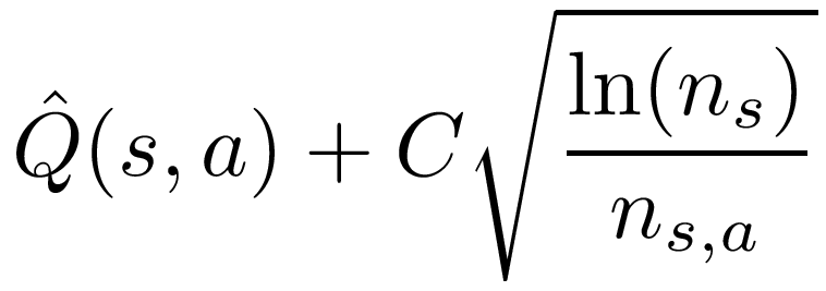
Computing UCB weights requires us to keep track not only of the estimated Q-values, but also the number of times each (state, action) pair has been seen. Analagous to Q-values, we don't need to keep track of visits to each state, because we can compute as the sum of the state's action's visits.
UCB weight can be used to select actions during exploration in two different ways. In lab 4, we selected an option randomly with probability proportional to the UCB weights. On the other hand, Monday's reading suggests deterministically selecting the action with the highest UCB weight. You should try out both of these methods to see which works best.
In UCBAgents.py, you need to finish implementing the class UCB_QLearningAgent. Luckily, much of the work is already done, since the class inherits from lab 5's QLearningAgent. The getAction method has been implemented for you, and calls the new method UCB_choice which you will need to implement. UCB_choice computes UCB weights for each legal action from the current state and then returns either the max-weight action, or a random action drawn with probability proportional to weights. You should test both versions to see which is more effective in each environment.
You can run your UCB_QLearningAgent on both the gridworld and PacMan domains with the following commands.
python gridworld.py -a q -k 100 -g TallGrid -u UCB_QLearningAgent

python pacman.py -p PacmanUCBAgent -x 2000 -n 2010 -l smallGrid
Remember from last week that both domains have a number of available layouts.
Next, you'll be taking things a step further and using MCTS to solve the MDP. Interestingly, MDP solving (not complete-information game playing) was the original purpose for which the UCT algorithm was proposed.
In lab 4, we used MCTS to make online decisions, where the agent ran MCTS at every node where it needed to make a decision. For this lab, you will first implement MCTS for offline learning, where the agent will explore and learn values using MCTS, but will then freeze its value estimates and use a greedy policy for testing.
The OfflineMCTSAgent class you will be implementing inherits from UCB_QLearningAgent, so selection and expansion are already implemented by getAction. In addition, the update function for OfflineMCTSAgent has been implemented for you. Your task is to implement backpropagation for Monte Carlo tree search. Note that because we do not have separation between the agent's environment and a simulator of that environment, we are omitting the simulation step. However, the result of repeated expansion operations on new states has an effect similar to simulation, albeit with higher memory overhead.
In Monte Carlo tree search, we don't update the value esimates at every timestep, so the update function that has been provided for you simply appends observations to a history list for later use. The backpropagation function gets called when a terminal state is encountered. At this point the value estimate of every (state, action) pair encountered in the rollout gets updated. Unlike Q-learning, there is no learning rate parameter, so the value estimate is simply the average (discounted) future reward across all instances where a (state, action) pair was encountered.
To update the value, you first need to calculate the discounted reward received over the rest of the rollout after the state and action were visited. For a state and action encountered at time T, the discounted future reward is
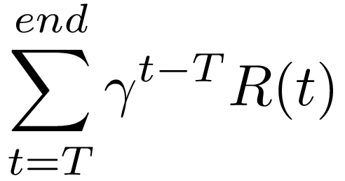
where gamma is the discount rate, and R(t) is the reward at time t. The best way to compute this sum is to work backwards from the last state and action in the rollout, accumulating the future reward after each time step. On every time step, the future reward is discounted, and the current reward added in. The following example demonstrates how the discounted reward is calculated.
Suppose that Pac-Man is in the smallGrid world with just two pieces of food. On every time step his living reward is -1. When he eats a piece of food he gets an additional reward of 10. If he manages to eat all the food he gets a bonus reward of 500. Given this setup, here is one example reward history he could have:
self.rewards = [-1, -1, 9, -1, -1, 509]Then his discounted reward for each step would be calculated as follows (assuming the discount is d):
discountedReward5 =  509
discountedReward4 = -1 + d*509
discountedReward3 = -1 + d*-1 + d2*509
discountedReward2 =  9 + d*-1 + d2*-1 + d3*509
discountedReward1 = -1 + d*9 + d2*-1 + d3*-1 + d4*509
discountedReward0 = -1 + d*-1 + d2*9 + d3*-1 + d4*-1 + d5*509
Each of these discounted rewards can be written in terms of the previous one like this:
discountedReward5 =  509
discountedReward4 = -1 + d * discountedReward5
discountedReward3 = -1 + d * discountedReward4
discountedReward2 =  9 + d * discountedReward3
discountedReward1 = -1 + d * discountedReward2
discountedReward0 = -1 + d * discountedReward1
In general the calculation is:
discountedRewardt = R(t) + d * discountedRewardt+1Thus if you iterate over the self.rewards list in reverse order, you can easily calculate the discounted reward for each time step. For this particular example the discounted rewards would be:
discountedReward5 = 509
discountedReward4 = 457
discountedReward3 = 410
discountedReward2 = 378
discountedReward1 = 340
discountedReward0 = 305
To correctly update the Q-value, we need to know the number of times each state/action pair was encountered in the current rollout. Call this value the new n_s,a. We also need to know the number of times the pair was seen across all previous rollouts; call this the old n_s,a. The new count can be determined by the number of times (s,a) appears in the history list. The old count is the difference between the total nubmer of visits to (s,a) and the new count. Updating the average value then works as follows:
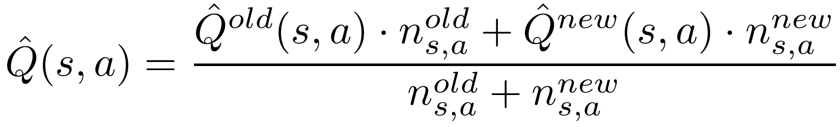
Where the new Q is the average discounted future reward across all occurrences of (s,a) in the current rollout, and the old Q is stored in the values table.
After all value estimates have been updated, backpropagation should reset self.history to an empty list for the start of the next rollout.
Use the following commands to run your offline MCTS agent on the Grid World and PacMan domains. remember there are many other options for the grids (-g and -l respectively).
python gridworld.py -a q -k 100 -g TallGrid -u OfflineMCTSAgent

python pacman.py -p PacmanMCTSAgent -x 2000 -n 2010 -l smallGrid
In contrast to the offline version, which starts all rollouts from the start state of the MDP, an online Monte Carlo tree search agent runs simulated rollouts from every node where it needs to make a decision. This requires access to a simulator that can predict the outcomes of those actions. The new version of gridworld.py and the new file pacmanSimulator.py each implement such a simulator, providing three methods:
Your task is to implement all four phases MCTS: selection, expansion, simulation, and backpropagation. Because OnlineMCTSAgent inherits from OfflineMCTSAgent, you have access to the UCB_choice and backpropagation methods you've already written, which should work without modification here.
Selection and expansion are in principle similar to getAction in the UCB_QlearningAgent, but need to make calls to simulator.nextState to get new states, and need to add each observation to the history list. The simulation phase begins after a new (state, action) pair has been expanded and runs the remainder of the rollout by calling simulator.rollout with the remaining number of steps.
When backpropagation is called, the history list should include (state, action, reward) tuples for each element of the selection path. All rewards from the simulation phase compressed into the final entry for the expanded state/action. That is the reward in self.history[-1] will be the reward at the expanded (state, action) pair, plus the sum of discounted rewards over the whole simulation phase.
The MCTS function puts all of the pieces together. This is the function called by getAction, but it does not need to return an action. Instead, it updates the values table, after which getAction calls computeActionFromQValues to pick the best action according to the simulation estimates. MCTS runs a number of rollouts determined by the self.rollouts field. Each rollout consists of selection, expansion, simulation, and backpropagation phases. The self.rollout_steps field gives the maximum number of actions that should be taken over the course of a rollout (including selection, expansion, and simulation phases). A rollout ends when either a terminal state or this depth limit is reached, regardless of which phase the algorithm is in.
You can test your online MCTS agent on gridworld or pacman with commands like the following.
gridworld.py -a q -k 50 -g TallGrid -u OnlineMCTSAgent -d 0.9
git add UCBAgents.py
git commit -m "final version"
git push