Week 9: searching

Monday

This week is searching and next week is sorting. For both of these topics there are multiple algorithms to accomplish the task (searching and/or sorting data). In addition to learning and coding a few searching and sorting algorithms, we are going to start analyzing algorithms. By this I mean classifying algorithms into broad categories so we can compare one algorithm versus another.

three algorithms to compare

To start I’ve got three algorithms to consider, which I am calling the handshake algorithm, the introductions algorithm, and the divide by 2 algorithm. Here are short descriptions of each:

handshake: suppose I have a class full of 34 students, and I want to meet each of my students. To do this, I walk around and say "Hi, I’m Jeff" to each student and shake their hand.
introductions: suppose I now want to introduce each student to every other student in the class. I start by taking the first student around to every other student and introducing them. Then I go back and get the second student, take them to every other student (minus the first one, since they’ve already met), and introduce them, and so on…
divide by 2: suppose I divide my class into two equal parts (17 students on each side of the room), then (not sure why..) get rid of one half and repeat the process. This time I divide my 17 remaining students in half as best I can (8 on one side of the room, 9 on the other side) and again get rid of one half. I now repeat this process over and over until I have just one student left.

When deciding which algorithm to use, programmers are usually interested in three things: run time, memory usage, and storage required (disk space). If your program takes too long to run, or needs more memory than the computer has, or needs more data than can fit on the hard drive, that’s a problem.

For this class, when analyzing algorithms, we will just focus on how many "steps" or operations each algorithm requires. For the handshake algorithm above, it will obviously require 34 handshakes if I have 34 students in my class. However, to classify this algorithm, I would really like to know how the number of handshakes changes as I change the number of students in my class. For example, here’s a simple table showing number of students vs number of handshakes:

number of students	number of handshakes
34	34
68	68
136	136
272	272

Hopefully it is obvious that, if the number of students doubles, the number of handshakes also doubles, and the number of handshakes is directly proportional to the number of students.

linear algorithms: O(N)

The handshake algorithm is an example of a linear algorithm, meaning that the number of steps required, which is ultimately related to the total run time of the algorithm, is directly proportional to the size of the data.

If we have a python list L of students (or student names, or integers, or whatever), where N=len(L), then, for a linear algorithm, the number of steps required will be proportional to N.

Computer scientists often write this using "big-O" notation as O(N), and we say the handshake algorithm is an O(N) algorithm (the O stands for "order", as in the "order of a function" — more on this below).

An O(N) algorithm is also called a linear algorithm because if you plot the number of steps versus the size of the data, you’ll get a straight line, like this:

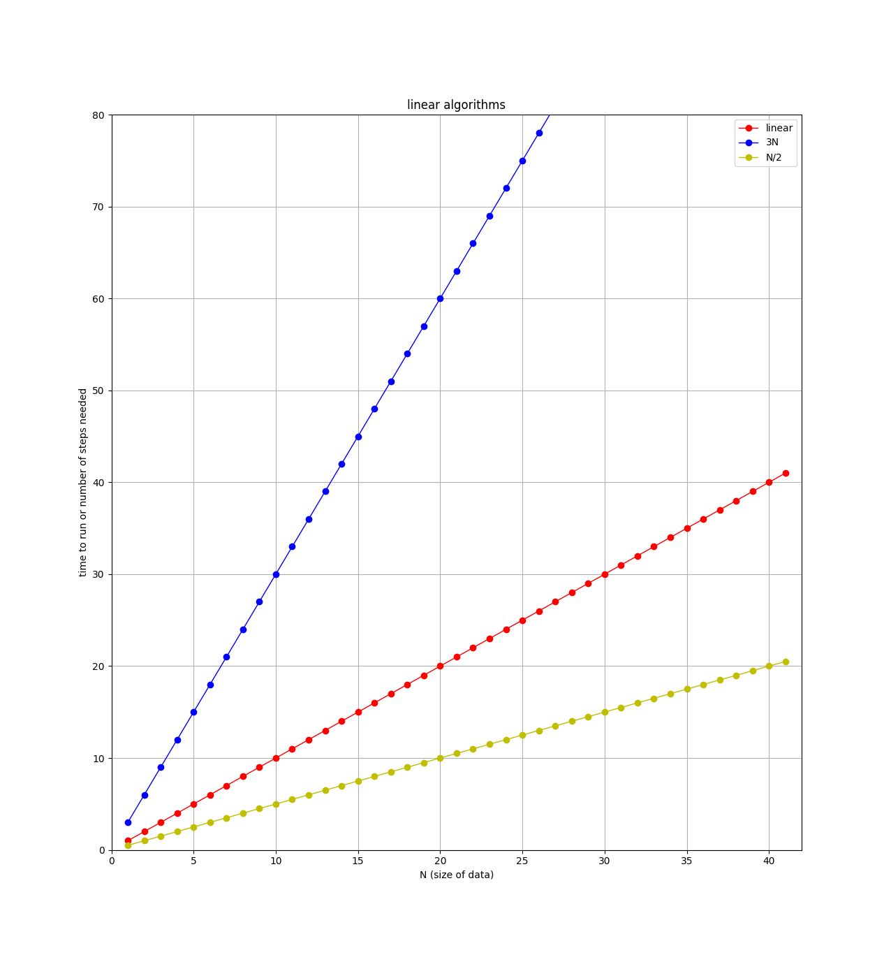
Note on the plot that there are 3 straight lines. When comparing algorithms, you might have one algorithm that requires N steps, and another that requires 3*N steps. For example, if I modify the handshake algorithm to not only shake the student’s hand, but also ask them where they are from, and write down their email address, then this algorithm requires 3 steps (shake, ask, write down) for each student. So for N students, there would be 3*N total steps. Clearly the algorithm that requires the least steps would be better, but both of these algorithms are classified as "linear" or O(N). When classifying algorithms and using the big-O notation, we will ignore any leading constants. So algorithms with 3*N steps, N steps, N/2 steps, and 100*N steps are all considered as "linear".

linear search

When searching for an item in a list, a simple search involves looking at each item in the list to see if it is the one you want. Here’s a function to search for x in a list L:

def linearSearch(x,L):
   """return True if x is found in L, False if not"""
   for item in L:
      if item == x:
         return True

   # if we get here, past the for loop, x is not in L
   return False

The function above only says if the item we are looking for is in the list or not. Other searches might be interested in where the item is in the list (if at all), or how many of the item are in the list. All of these are examples of O(N) algorithms.

Can you think of other O(N) algorithms we have used this semester?

quadratic algorithms: \$O(N^2)\$

For the introduction algorithm discussed above, how many introductions are required? We can count them and look for a pattern. For example, suppose I had only 6 students, then the number of introductions would be:

5 + 4 + 3 + 2 + 1 = 15

Remember, the first student is introduced to all of the others (5 intros), then the second student is introduced to all of the others, minus the first student, since they already met (4 intros), and so on.

If I had 7 students, then the number of introductions would be:

6 + 5 + 4 + 3 + 2 + 1 = 21

and if I had N students:

(N-1) + (N-2) + (N-3) + ... + 3 + 2 + 1 = ???

If you can see the pattern, awesome! Turns out the answer is \$\frac{(N-1)(N)}{2}\$ introductions for a class of size N. Try it for the N=6 and N=7 cases:

>>> N=6
>>> (N/2)*(N-1)
15.0
>>> N=7
>>> (N/2)*(N-1)
21.0

Another way to see that is with a bar chart showing how many introductions each student will make:

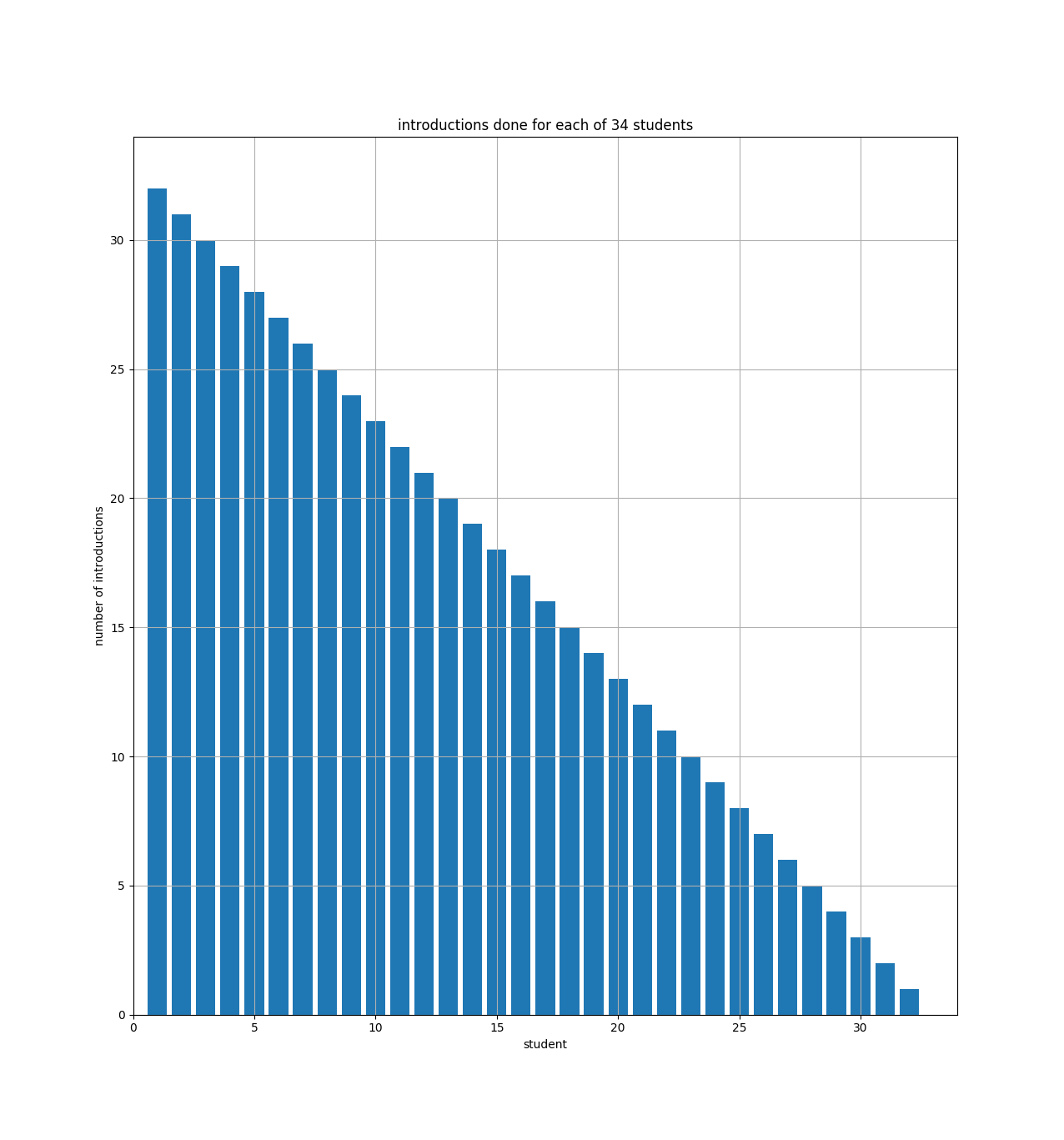
The bar chart just shows that student number 1 (on the x axis) has to do 33 introductions (the y axis), and student number 2 has to do 32, etc. And you can see how the bars fill up half of a 34x34 square. So if we had N students, the bar chart would fill up half of an NxN square.

For the equation above (\$\frac{(N-1)(N)}{2}\$), if you multiply it out, the leading term is N-squared over 2 (i.e., half of an NxN square).

When comparing algorithms, we are mostly concerned with how they will perform when the size of the data is large. For the introductions algorithm, the number of steps depends directly on the square of N. This is written in big-O notation as \$O(N^2)\$ (order N squared). These types of algorithms are called quadratic, since the number of steps will quadruple if the size of the data is doubled.

Here’s a table showing the number of introductions versus the number of students in my class:

number of students	number of introductions
34	561
68	2278
136	9180
272	36856

Notice how the number of introductions goes up very quickly as the size of the class is increased (compare to number of handshakes above).

logarithmic algorithms: `O(logN)`

For the divide by 2 algorithm discussed above, how many times can I divide my class in two before I get down to just one student left?

To make things easier, assume I have a class of just 32 students. Then I can divide the students in two 5 times: 32→16→8→4→2→1.

We’re interested in knowing how the number of steps changes as the size of the data changes. If I double my class size to 64 students, how many more steps (divisions) will be required? The answer: just one extra division! That’s because the first division (64→32) gets us back to the class of just 32 students, and we know that only took 5 divisions, so a class of 64 will take 6 total divisions.

Again, if you can see the pattern here, awesome! If not, maybe this table will help:

number of students	number of divisions
32	5
64	6
128	7
256	8

Hopefully you can see that 2 raised to the 5th power is 32, and 2 to the 6th is 64 (try it in the python interactive shell: 2**5).

So for a class of N students, we want to know what x is in the equation 2**x=N. This is easily solved with a logarithm. Taking the base 2 log of N will get you x, which you can also see using the python interactive shell:

>>> from math import log
>>> log(32,2)
5.0
>>> log(64,2)
6.0
>>> log(128,2)
7.0
>>> log(1000000,2)
19.931568569324174

binary search: O(logN)

The binary search, which we will look at on Wednesday, is an example of a divide by 2 algorithm. Here’s a table showing the number of steps required for a linear algorithm (linear search) and a logarithmic algorithm (binary search). If you could use either one, and the size of your data was large, which would you choose?

N (size of list)	O(N) steps	O(logN) steps
1000000	1000000	19.9
2000000	2000000	20.9
4000000	4000000	21.9

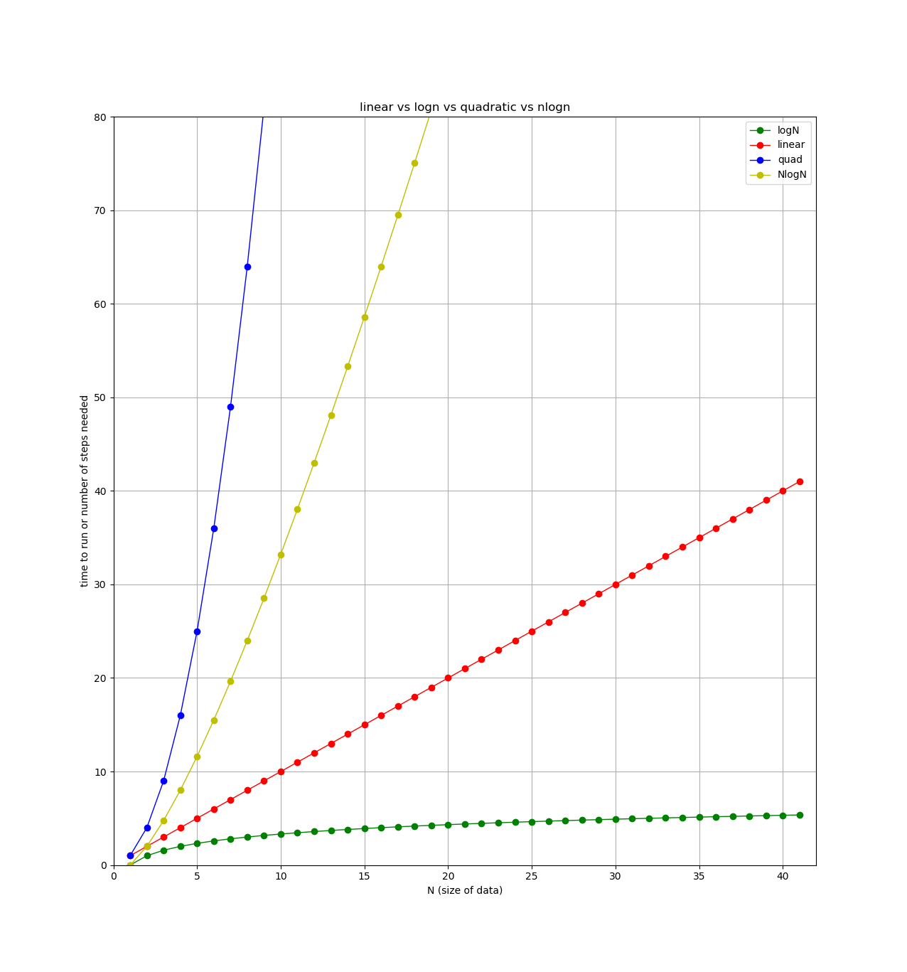
Finally, here’s a plot showing each type of algorithm we’ve looked at so far (plus one more we’ll see next week). All lines show number of steps (y axis) versus the size of the data (x axis).

Wednesday: binary search

If our data is already sorted from low to high, is there a better way to search for x in L?

L = [5, 16, 33, 34, 60, 89]

If we are searching for x=20, there is no point searching past the 33, since we know the list is sorted from low to high, and we are already past what we are looking for.

Here is another example: if I say "I am thinking of a number from 1 to 100", and that when you guess, I will tell you if you are too high or too low, what is the first number you would guess?

A linear search would guess one number at a time, from 1 to 100.

A binary search would pick the middle and first guess 50. If that is too low, we can then concentrate on the upper half (51-100), and we have already eliminated half of the list! In a binary search, each guess should split the remaining list in half, and eliminate one half.

binary search pseudo code

Here is the pseudo-code for binary search:

set low = lowest-possible index
set high = highest possible index
LOOP:
    calculate middle index = (low + high)//2
    if item is at middle index, we are done (found it! return True)
    elif item is < middle item,
       set high to middle index - 1
    elif item is > middle item,
       set low to middle index + 1
    if low is greater than high, item not here (done, return False)

And here is an example of how the low, mid, and high indices change as the search is happening:

x = 99
L = [-20, -12, -4, 1, 7, 44, 45, 46, 58, 67, 99, 145]
index: 0    1   2  3  4   5   6   7   8   9  10   11

low	high	mid	L[mid]	explanation
0	11	5	44	x is > 44, so low becomes mid+1 (6)
6	11	8	58	x is > 58, so low becomes mid+1 again (9)
9	11	10	99	x is == 99, so return `True`

And here is an example where the item we are searching for is not in the list. The search keeps going until low is greater than the high index.

x = -10
L = [-20, -12, -4, 1, 7, 44, 45, 46, 58, 67, 99, 145]
index: 0    1   2  3  4   5   6   7   8   9  10   11

low	high	mid	L[mid]	explanation
0	11	5	44	x is < 44, so high becomes mid-1 (4)
0	4	2	-4	x is < -4, so high becomes mid-1 again (1)
0	1	0	-20	x is > -20, so low becomes mid+1 (1)
1	1	1	-12	x is > -12, so low becomes mid+1 (2)
2	1			low is > high, so return `False`

add your search function to `searches.py`

Let’s write our two search functions, linearSearch(x,L) and binarySearch(x,L), in a file called searches.py. Then we can import this file and use those functions in other programs. If we put these two functions in a file called searches.py, then we can say from searches import * in other programs and be able to use those two search functions!

Here is the start of searches.py, with the linearSearch(x,L) function in it. Note the test code at the bottom of the file:

def linearSearch(x,L):
   """return True if x is in L, False if not"""

   for item in L:
      if item == x:
         return True

   # only gets here if not found!
   return False

if __name__ == "__main__":
   # put test code here
   L = range(10)
   x = 5
   print(x, L, linearSearch(x,L))
   x = 500
   print(x, L, linearSearch(x,L))

The if __name__ == "__main__": part just decides if this searches.py file is being imported or run. If it is being run, like python3 searches.py, then we want to run the test code. If it is being imported, to be used in another program, then we do not want to run the test code (if we are importing it, we assume it already works!).

write a program that imports `searches.py`

Here’s a program that reads in the wordlist we have used before (in /usr/share/dict/words) and then asks the user for a word. Once we have a word from the user, we can use our binarySearch(x,L) function to check if it’s a valid word.

Here’s a run of the program:

$ python3 words.py
word to search for: hello
FOUND!
word to search for: zebra
FOUND!
word to search for: skdjfkldjfl
word to search for:
$

And here’s the source code:

from searches import *

def main():
  words = readFile("/usr/share/dict/words")
  done = False
  while not done:
    word = input("word to search for: ")
    if word == "":
      done = True
    else:
      if binarySearch(word, words):
        print("FOUND!")

def readFile(filename):
  """read in words from file, return as a list"""
  words = []
  infile = open(filename, "r")
  for line in infile:
    words.append(line.strip())
  infile.close()
  return words

main()

Friday

In algorithms.py are some simple loops and code snippets (see below). Can you figure out the order of each? For example, is the first one O(N) or \$O(N^2)\$?

# How many "steps" for each of the following?
# What happens to the number of steps when n --> 2n?

# O(1), O(logN), O(N), O(NlogN), O(N**2)

#############################################
# 1
N = int(input("N: "))
for i in range(N):
   print(i)
#############################################
# 2
N = int(input("N: "))
for i in range(100):
   print(i*N)
#############################################
# 3
N = int(input("N: "))
for i in range(N):
   print(i)
for j in range(N):
   print(j)
#############################################
# 4
N = int(input("N: "))
for i in range(N):
   for j in range(N):
      print(i, j)
#############################################
# 5
N = int(input("N: "))
for i in range(N):
   for j in range(i,N):
      print(i, j)
#############################################
# 6
N = int(input("N: "))
for i in range(N):
   for j in range(10):
      print(i, j)
#############################################
# 7
N = int(input("N: "))
while N > 1:
   print(N)
   N = N/2
#############################################
# 8
L = [1,2,5,7,13,21,24,25,26,33,34,38,50,57,58,63]
N = len(L)
mid = N//2
print(L[mid])
#############################################
# 9
N = int(input("N: "))
for i in range(N):
   k = N
   while k > 1:
      print(i, k)
      k = k/2
#############################################