Week 9: Searching

At the start, the program should ask the user which mode to play the game in: easy or hard.
The game then chooses a random target number between 0 and 200.
The game should then repeatedly prompt the user for a guess of the number. It should check the user’s number against the target. If they match, the user has won and the game ends. Otherwise:
- In easy mode, tell the user whether the target is lower or higher than the value they entered.
- In hard mode, just tell the user whether the guess was right or wrong, but don’t give any additional hints or feedback.

Design

To practice top-down design, start by working with a neighbor to design your main() function and sketch out all the functions that main() will need to call. Be sure to consider the types of all function parameters and return values, noting them in comments associated with each function.

Implementation

After you have completed the design, implement the program and test it.

Bonus

If you finish early, think about how you might add another game mode: either extra easy or extra hard, and implement one such mode if time permits.

Wednesday

Search Motivation

Computer Science as a discipline is focused on two primary questions:

What types of problems can be solved computationally?
How efficiently can these problems be solved?

One of the core problems we computers are asked to solved is the search problem. Broadly speaking, the search problem searches for a query item in a potentially large set of potential matches. For two large internet companies, search is one part of their core business model.

Searching efficiently can help you solve larger problems, help more customers, or make larger profits. So how do we organize data and write code/algorithms to search efficiently? And what do we even mean by efficient?

As concrete examples, Google once found that a half-second delay caused a 20% drop in traffic, and 100 extra milliseconds of page load time reduced Amazon’s revenue substantially.

Consider the two game modes in your number guessing game — the modes differ slightly in how they give you feedback when your guess is wrong. Try playing both games. Do you have a different strategy for one game than the other? Why?

Algorithmic Complexity

In addition to learning and coding a few searching and sorting algorithms over the next two weeks, we’ll also start analyzing algorithms. We can analyze and compare algorithms by classifying them into broad complexity categories so we can compare one type of algorithm to another without worrying about details like implementation language used or speed of the physical machine.

To analyze the complexity of an algorithm, we need to consider several questions. For now, we’ll think about these in the context of searching, but these idea apply much more generally too:

What are the resources are we trying to optimize for? (e.g., minimize time to win the game, minimize CPU time, minimize memory usage)
How do we analyze how long it takes for an algorithm to finish?
If we want to count the "steps" needed to complete a task, what counts as a step? (e.g., number of guesses, number of comparisons made in a search)
Do we care about the best case scenario, what happens on average, or the worst case?

Let’s draw a rough analysis of our guessing game on the board.

Three algorithms to compare

To start I’ve got three algorithms to consider, which I am calling the handshake algorithm, the introductions algorithm, and the RPS algorithm. Here are short descriptions of each:

Handshake: suppose I have a class full of 34 students, and I want to meet each of my students. To do this, I walk around and say "Hi, I’m Kevin" to each student and shake their hand.
Introductions: suppose I now want to introduce each student to every other student in the class. I start by taking the first student around to every other student and introducing them. Then I go back and get the second student, take them to every other student (minus the first one, since they’ve already met), and introduce them, and so on…
Rock, Paper, Scissors (RPS): suppose we decide to hold a class-wide rock, paper, scissors tournament, so we divide the class into two equal parts (17 students on each side of the room), then after the first round of winners is decided, we eliminate one half of the students and repeat the process. This time we divide the 17 remaining students in half as best we can (8 on one side of the room, 9 on the other side) and we play another RPS round to eliminate another half. We then repeat this process over and over until we have just one student left, the tournament winner.

When deciding which algorithm to use, programmers are usually interested in three things: run time, memory usage, and storage required (disk space). If your program takes too long to run, or needs more memory than the computer has, or needs more data than can fit on the hard drive, that’s a problem.

For this class, when analyzing algorithms, we will just focus on how many "steps" or operations each algorithm requires. For the handshake algorithm above, it will obviously require 34 handshakes if I have 34 students in my class. However, to classify this algorithm, I would really like to know how the number of handshakes changes as I change the number of students in my class. For example, here’s a simple table showing number of students vs number of handshakes:

number of students	number of handshakes
34	34
68	68
136	136
272	272

Hopefully it is obvious that, if the number of students doubles, the number of handshakes also doubles, and the number of handshakes is directly proportional to the number of students.

Linear algorithms: O(N)

The handshake algorithm is an example of a linear algorithm, meaning that the number of steps required, which is ultimately related to the total run time of the algorithm, is directly proportional to the size of the data.

If we have a python list L of students (or student names, or integers, or whatever), where N=len(L), then, for a linear algorithm, the number of steps required will be proportional to N.

Computer scientists often write this using "big-O" notation as O(N), and we say the handshake algorithm is an O(N) algorithm (the O stands for "order", as in the "order of a function").

An O(N) algorithm is also called a linear algorithm because if you plot the number of steps versus the size of the data, you’ll get a straight line, like this:

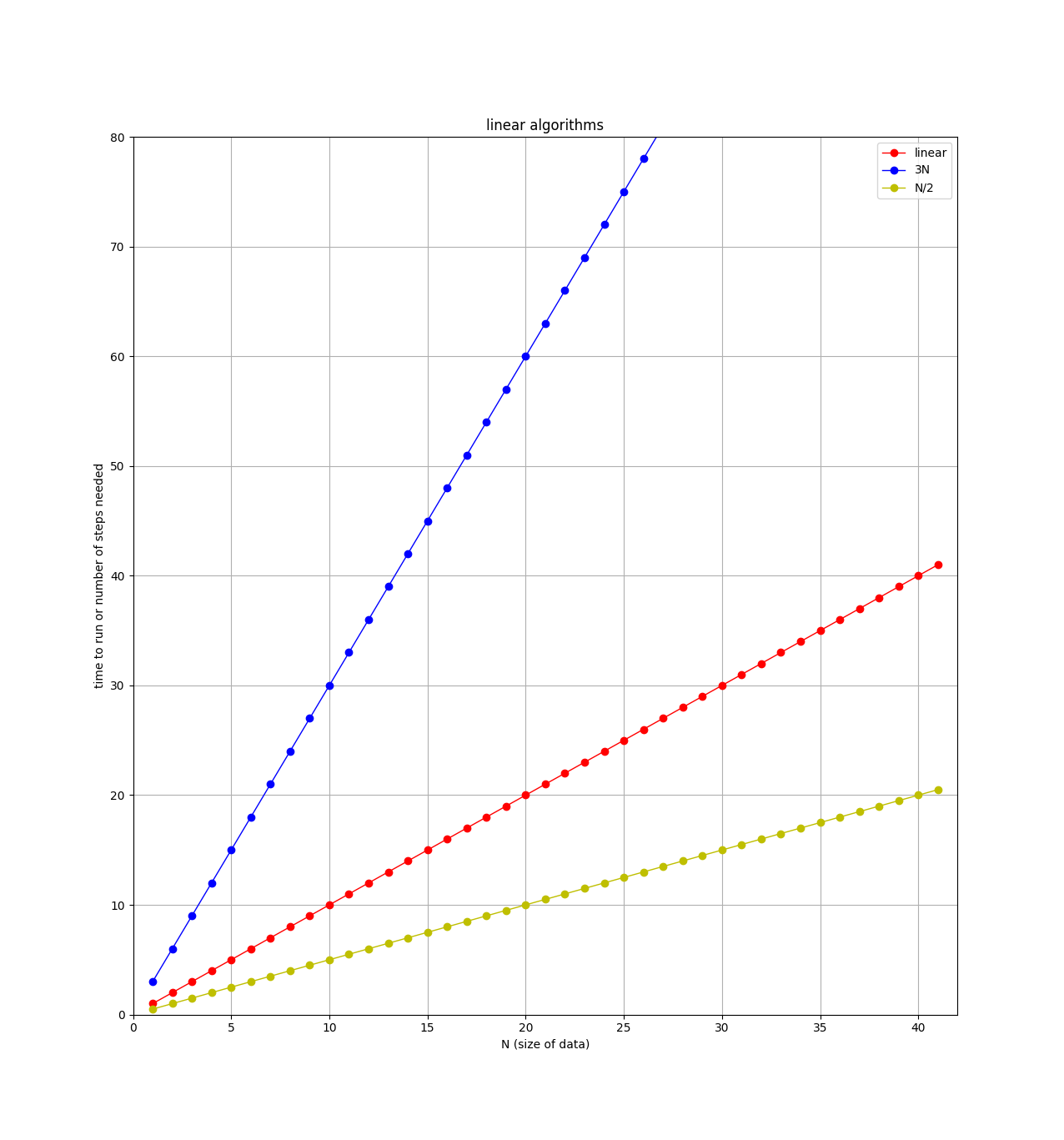
Note on the plot that there are 3 straight lines. When comparing algorithms, you might have one algorithm that requires N steps, and another that requires 3*N steps. For example, if I modify the handshake algorithm to not only shake the student’s hand, but also ask them where they are from, and write down their email address, then this algorithm requires 3 steps (shake, ask, write down) for each student. So for N students, there would be 3*N total steps. Clearly the algorithm that requires the least steps would be better, but both of these algorithms are classified as "linear" or O(N). When classifying algorithms and using the big-O notation, we will ignore any leading constants. So algorithms with 3*N steps, N steps, N/2 steps, and 100*N steps are all considered as "linear".

Quadratic Algorithms: \$O(N^2)\$

For the introduction algorithm discussed above, how many introductions are required? We can count them and look for a pattern. For example, suppose I had only 6 students, then the number of introductions would be:

5 + 4 + 3 + 2 + 1 = 15

Remember, the first student is introduced to all of the others (5 intros), then the second student is introduced to all of the others, minus the first student, since they already met (4 intros), and so on.

If I had 7 students, then the number of introductions would be:

6 + 5 + 4 + 3 + 2 + 1 = 21

and if I had \$N\$ students:

\$(N-1) + (N-2) + (N-3) + ... + 3 + 2 + 1 =\$ ???

If you can see the pattern, awesome! Turns out the answer is \$\frac{(N-1)(N)}{2}\$ introductions for a class of size N. Try it for the N=6 and N=7 cases:

>>> N=6
>>> (N/2)*(N-1)
15.0
>>> N=7
>>> (N/2)*(N-1)
21.0

Another way to see that is with a bar chart showing how many introductions each student will make:

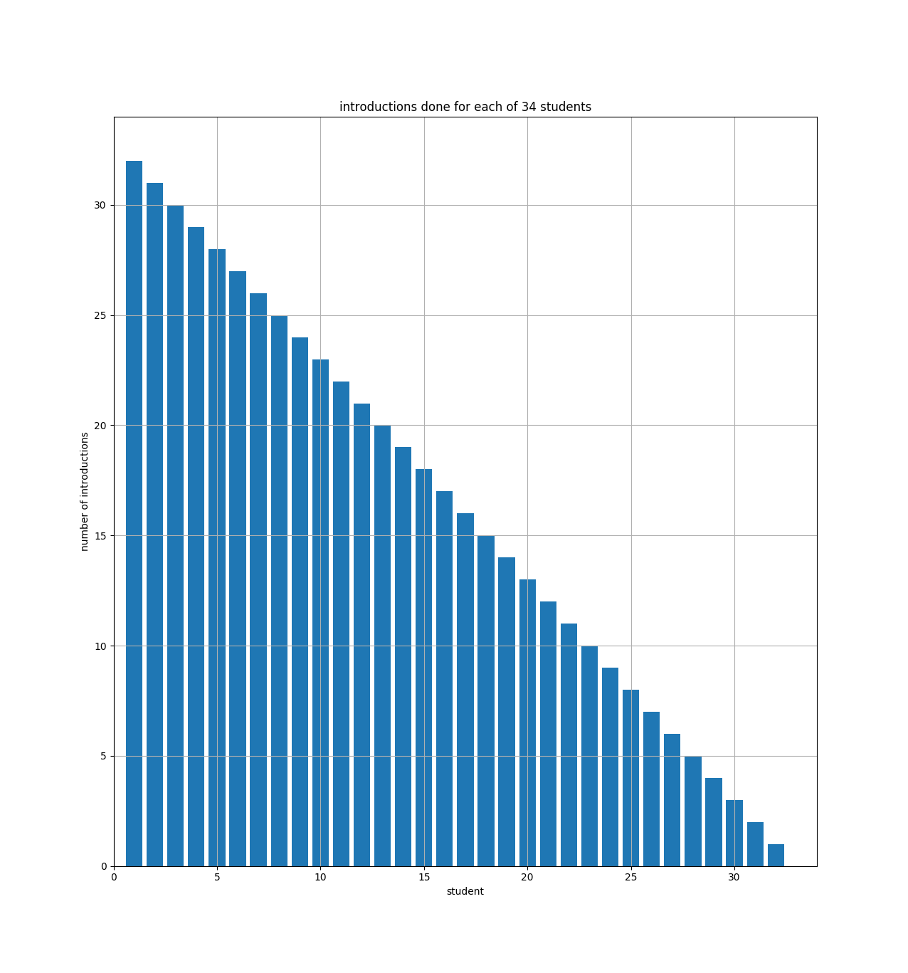
The bar chart just shows that student number 1 (on the x axis) has to do 33 introductions (the y axis), and student number 2 has to do 32, etc. And you can see how the bars fill up half of a 34x34 square. So if we had N students, the bar chart would fill up half of an NxN square.

For the equation above \$\frac{(N-1)(N)}{2}\$, if you multiply it out, the leading term is N-squared over 2 (i.e., half of an NxN square).

When comparing algorithms, we are mostly concerned with how they will perform when the size of the data is large. For the introductions algorithm, the number of steps depends directly on the square of N. This is written in big-O notation as \$O(N^2)\$ (order N squared). These types of algorithms are called quadratic, since the number of steps will quadruple if the size of the data is doubled.

Here’s a table showing the number of introductions versus the number of students in my class:

number of students	number of introductions
34	561
68	2278
136	9180
272	36856

Notice how the number of introductions goes up very quickly as the size of the class is increased (compare to number of handshakes above).

Logarithmic algorithms: \$O(\log N)\$

For the RPS algorithm discussed above, how many times can I divide my class in two before I get down to just one student left?

To make things easier, assume I have a class of just 32 students. Then I can divide the students in two 5 times: 32→16→8→4→2→1.

We’re interested in knowing how the number of steps changes as the size of the data changes. If I double my class size to 64 students, how many more steps (divisions) will be required? The answer: just one extra division! That’s because the first division (64→32) gets us back to the class of just 32 students, and we know that only took 5 divisions, so a class of 64 will take 6 total divisions.

Again, if you can see the pattern here, awesome! If not, maybe this table will help:

number of students	number of divisions
32	5
64	6
128	7
256	8

Hopefully you can see that 2 raised to the 5th power is 32, and 2 to the 6th is 64 (try it in the python interactive shell: 2**5).

So for a class of N students, we want to know what x is in the equation 2**x=N. This is easily solved with a logarithm. Taking the base 2 log of N will get you x, which you can also see using the python interactive shell:

>>> from math import log
>>> log(32,2)
5.0
>>> log(64,2)
6.0
>>> log(128,2)
7.0
>>> log(1000000,2)
19.931568569324174

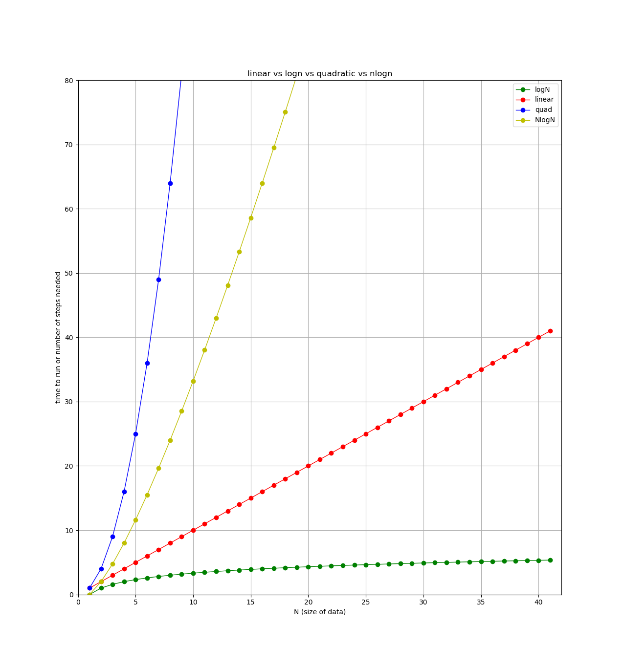
Finally, here’s a plot showing each type of algorithm we’ve looked at so far (plus one more we’ll see next week). All lines show number of steps (y axis) versus the size of the data (x axis).

Friday

Linear Search

To explore the complexity of search, we will narrow the problem to searching for an item x in a python list of items. Python already has two ways of doing this. The first is the Boolean in operator, x in ls which returns True if x is in the list ls and False otherwise. Python also supports the index() method which will tell you the position in the list of the first occurrence of x, provided x appears in the list. So ls.index(x) will return an integer position if x is in ls. If x is not in the list, Python will generate an error called an exception that will likely crash your program since we have not talked much about how to handle exceptions in this class.

But how do these methods actually work? At some point, a computer scientist and python programmer designed and wrote the code for these built-in features. We will discuss the algorithm for searching a collection of items. Together, we’ll write a function that does something familiar: search through a list for an item without using the in operator. Our functions will be called contains and position_of.

Binary Search

A key algorithmic question is: can we do better? In some cases, we can’t (and we can prove this!). In the case of linear search, we cannot do better in the general case. However, if all items in the collection are in sorted order, we can perform a faster algorithm known as binary search.

Binary search works using divide and conquer approach. Each step of the algorithm divides the number of items to search in half until it finds the value or has no items left to search. Here is some pseudocode for the algorithm:

set low = lowest-possible index
set high = highest possible index
LOOP:
    calculate middle index = (low + high) // 2
    if item is at middle index, we're done (found it! return matching index)
    elif item is < middle item,
      set high to middle - 1
    elif item is > middle item,
      set low to middle + 1
if low is ever greater than high, item not here (done, return -1)